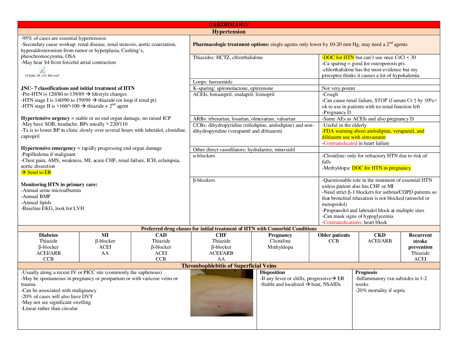
Statistics > STUDY GUIDE > National University College, STATISTICS - STAT MISC NEW TEST BANK FOR CHAPTER 1 TO CHAPTER 7: CONTAI (All)
National University College, STATISTICS - STAT MISC NEW TEST BANK FOR CHAPTER 1 TO CHAPTER 7: CONTAINS STUDENT'S ANSWER & VERIFIED CORRECT ANSWER; A+ WORK.
Document Content and Description Below
Chapter 1 • Question 1 1 out of 1 points Classify the following variable as either nominal or continuous: age. • Question 2 0 out of 1 points Classify the fol... lowing variable as either nominal or continuous: gender. • Question 3 1 out of 1 points Classify the following variable as either nominal or continuous: height. • Question 4 1 out of 1 points Classify the following variable as either nominal or continuous: race. • Question 5 1 out of 1 points A café owner decided to calculate how much revenue he gained from lattes each month. What type of variable would the amount of revenue gained from lattes be? • Question 6 1 out of 1 points A café owner wanted to compare how much revenue he gained from lattes across different months of the year. What type of variable is 'month'? • Question 7 1 out of 1 points Which of the following best describes a confounding variable? • Question 8 1 out of 1 points A demand characteristic is: A personality trait that affects the results of an experiment in an undesirable way. When the experimenter's behavior affects the results of an experiment. When a person responds in an experiment in a way that is consistent with their beliefs about how the experimenter would like them to behave. A personality trait that makes a participant likely to find an experiment too demanding. • Question 9 1 out of 1 points If a test is valid, what does this mean? The test has internal consistency. The test will give consistent results. The test measures a useful construct or variable. The test measures what it claims to measure. • Question 10 1 out of 1 points When questionnaire scores predict or correspond with external measures of the same construct that the questionnaire measures it is said to have: Factorial validity Criterion validity Ecological validity Content validity • Question 11 1 out of 1 points When the results of an experiment can be applied to real-world conditions, that experiment is said to have: Factorial validity Criterion validity Ecological validity Content validity • Question 12 1 out of 1 points A variable manipulated by a researcher is known as: An independent variable A dependent variable A confounding variable A discrete variable • Question 13 1 out of 1 points A variable that measures the effect that manipulating another variable has is known as: An independent variable A dependent variable A confounding variable A predictor variable • Question 14 1 out of 1 points A predictor variable is another name for: An independent variable A dependent variable A confounding variable A discrete variable • Question 15 1 out of 1 points The discrepancy between the numbers used to represent something that we are trying to measure and the actual value of what we are measuring is called: Reliability Measurement error The 'fit' of the model Variance • Question 16 1 out of 1 points What kind of variable is IQ, measured by a standard IQ test? Discrete Categorical Nominal Continuous • Question 17 1 out of 1 points A frequency distribution in which low scores are most frequent (i.e. bars on the graph are highest on the left hand side) is said to be: Negatively skewed Leptokurtic Positively skewed Platykurtic • Question 18 1 out of 1 points A frequency distribution in which high scores are most frequent (i.e. bars on the graph are highest on the right hand side) is said to be: Negatively skewed Leptokurtic Positively skewed Platykurtic • Question 19 1 out of 1 points A frequency distribution in which there are too many scores at the extremes of the distribution said to be: Negatively skewed Leptokurtic Positively skewed Platykurtic • Question 20 1 out of 1 points A frequency distribution in which there are too few scores at the extremes of the distribution said to be: Negatively skewed Leptokurtic Positively skewed Platykurtic • Question 21 1 out of 1 points Which of the following is designed to compensate for practice effects? A repeated measured design Counterbalancing A control condition Giving participants a break between tasks • Question 22 1 out of 1 points Variation due to variables that have not been measured is known as: Unsystematic variation Homogenous variance Systematic variation Residual variance • Question 23 1 out of 1 points The purpose of a control condition is to: Allow inferences about cause. Control for participant characteristics. Show up relationships between predictor variables. Rule out a tertium quid. • Question 24 1 out of 1 points If the scores on a test have a mean of 26 and a standard deviation of 4, what is the z-score for a score of 18? 2 11 -2 -1.41 • Question 25 1 out of 1 points What is a scientific journal? A piece of scientific research that has not yet been published. A notebook kept by scientists containing important details of all their own experimental research for future reference. A collection of articles written by scientists that have been peer reviewed. A collection of articles written by scientists that have not yet been reviewed by other scientists in the field. • Question 26 1 out of 1 points The standard deviation is the square root of the: range variance sum of squares coefficient of determination • Question 27 1 out of 1 points Below is a histogram of ratings of Britney Spears's CD, Britney. What can we say about the data from this histogram? The data are leptokurtic. The data are normally distributed. The modal score is 5. The median rating was 2. • Question 28 1 out of 1 points What is the standard deviation? The variance squared. A measure of the dispersion or spread of data around the mean. The degree to which scores cluster at the ends of the distribution. A measure of the relationship between two variables. • Question 29 1 out of 1 points Complete the following sentence: A small standard deviation (relative to the value of the mean itself) (Hint: The standard deviation is a measure of the dispersion or spread of data around the mean.) indicates that the data points are distant from the mean. indicates that the mean is a poor fit of the data. indicates that you should analyze your data with a non-parametric test. indicates that data points are close to the mean (i.e. the mean is a good fit of the data). • Question 30 1 out of 1 points Complete the following sentence: A large standard deviation (relative to the value of the mean itself) (Hint: The standard deviation is a measure of the dispersion or spread of data around the mean.) indicates that the data points are distant from the mean (i.e. the mean is a poor fit of the data). indicates that the data points are close to the mean. indicates that the mean is a good fit of the data. indicates that you should analyze your data with a parametric test. Thursday, March 14, 2019 8:39:12 PM EDT Chapter # 2 • Question 1 1 out of 1 points 'Children can learn a second language faster before the age of 7'. Is this statement: A two-tailed hypothesis A non-scientific statement A one-tailed hypothesis A null hypothesis • Question 2 1 out of 1 points If my experimental hypothesis were 'Eating cheese before bed affects the number of nightmares you have', what would the null hypothesis be? Eating cheese before bed gives you more nightmares. The number of nightmares you have is not affected by eating cheese before bed. Eating cheese before bed gives you fewer nightmares. Eating cheese is linearly related to the number of nightmares you have. • Question 3 1 out of 1 points If my null hypothesis is 'Dutch people do not differ from English people in height', what is my alternative hypothesis? All of the statements are plausible alternative hypotheses. Dutch people are taller than English people. English people are taller than Dutch people. Dutch people differ in height from English people. • Question 4 1 out of 1 points Which of the following is true about a 95% confidence interval of the mean: 95% of population means will fall within the limits of the confidence interval. 95 out of 100 sample means will fall within the limits of the confidence interval. 95 out of 100 confidence intervals will contain the population mean. There is a 0.05 probability that the population mean falls within the limits of the confidence interval. • Question 5 1 out of 1 points What does a significant test statistic tell us? All of the above. There is an important effect. The hull hypothesis is false. That the test statistic is larger than we would expect if there were no effect in the population. • Question 6 1 out of 1 points Of what is p the probability? (Hint: NHST relies on fitting a 'model' to the data and then evaluating the probability of this 'model' given the assumption that no effect exists.) p is the probability of observing a test statistic at least as big as the one we have if there were no effect in the population (i.e., the null hypothesis were true). p is the probability that the results are due to chance, the probability that the null hypothesis (H0) is true. p is the probability that the results are not due to chance, the probability that the null hypothesis (H0) is false. p is the probability that the results would be replicated if the experiment was conducted a second time. • Question 7 1 out of 1 points A Type I error occurs when: (Hint: When we use test statistics to tell us about the true state of the world, we're trying to see whether there is an effect in our population.) We conclude that there is an effect in the population when in fact there is not. We conclude that there is not an effect in the population when in fact there is. We conclude that the test statistic is significant when in fact it is not. The data we have typed into SPSS is different from the data collected. • Question 8 1 out of 1 points A Type II error occurs when: (Hint: This would occur when we obtain a small test statistic--perhaps because there is a lot of natural variation between our samples.) We conclude that there is an effect in the population when in fact there is not. We conclude that there is not an effect in the population when in fact there is. We conclude that the test statistic is significant when in fact it is not. The data we have typed into SPSS is different from the data collected. • Question 9 1 out of 1 points If we calculated an effect size and found it was r = .21 which expression would best describe the size of effect? (Hint: The value of r can lie between 0 (no effect) and 1 (a perfect effect).) medium to large small large small to medium • Question 10 1 out of 1 points Power is the ability of a test to detect an effect given that an effect of a certain size exists in a population. True False • Question 11 1 out of 1 points We can use power to determine how large a sample is required to detect an effect of a certain size. Selected Answer: True True False • Question 12 1 out of 1 points Power is linked to the probability of making a Type I error. True False • Question 13 1 out of 1 points The power of a test is the probability that a given test is reliable and valid. True False • Question 14 1 out of 1 points The power of a statistical test depends on how big the effect actually is. True False • Question 15 1 out of 1 points The power of a statistical test depends on how strict we are about deciding that an effect is significant. True False • Question 16 1 out of 1 points The power of a statistical test depends on how strict we are about deciding that an effect is significant. True False • Question 17 1 out of 1 points The power of a statistical test does not depend on the sample size. True False • Question 18 1 out of 1 points The power of a statistical test depends on whether the test is a one- or two-tailed test. True False • Question 19 1 out of 1 points What is the null hypothesis for the following question: Is there a relationship between heart rate and the number of cups of coffee drunk within the last 4 hours? People who drink more cups of coffee will have significantly lower heart rates. People who drink more coffee will have significantly higher heart rates. There will be no relationship between heart rate and the number of cups of coffee drunk within the last 4 hours. There will be a significant relationship between the number of cups of coffee drunk within the last 4 hours and heart rate. • Question 20 1 out of 1 points What is the alternative hypothesis for the following question: Does eating salmon make your skin glow? Eating salmon does not predict the glow of skin. There will be no difference in the appearance of the skin of people who eat salmon compared to those who don't. People who eat salmon will have a more glowing complexion compared to those who don't. People who eat salmon will have a similar complexion to those who do not. • Question 21 1 out of 1 points 'Children can learn a second language differently before the age of 7 than after.' Is this statement: A two-tailed hypothesis A non-scientific statement A one-tailed hypothesis A null hypothesis • Question 22 1 out of 1 points What are variables? Variables are estimated from the data and are (usually) constants believed to represent some fundamental truth about the relations in the model. Variables are measured constructs that vary across entities in the sample. Variables estimate the centre of the distribution. Variables estimate the relationship between two parameters. • Question 23 1 out of 1 points What are parameters? All of the options describe parameters. Parameters are measured constructs that vary across entities in the sample. A parameter tells us about how well the mean represents the sample data. Parameters are estimated from the data and are (usually) constructs believed to represent some fundamental truth about the relations between variables in the model. • Question 24 1 out of 1 points Assume a researcher found that the correlation between a test she had developed and exam performance was .5 in a study of 25 students. She had previously been informed that correlations under .30 are considered unacceptable. The 95% confidence interval was [0.131, 0.747]. Can you be confident that the true correlation is at least 0.30? No you cannot, because the lower boundary of the confidence interval is .131, which is less than .30, and so the true correlation could be less than .30. Yes you can, because the upper boundary of the confidence interval is above .30 we can be 95% confident that the true correlation will be above .30 No you cannot, because the sample size was too small. Yes you can, because the correlation coefficient is .5 (which is above .30) and falls within the boundaries of the confidence interval. • Question 25 1 out of 1 points Under a null hypothesis, a sample value yields a p-value of .015. Which of the following statements is true? This finding is statistically significant at the .01 level of significance. This finding is statistically significant at the .05 level of significance. This finding is not statistically significant. This finding is statistically significant at the .001 level of significance. • Question 26 1 out of 1 points In general, as the sample size ( N) increases: The confidence interval becomes less accurate. The confidence interval gets wider. The confidence interval is unaffected. The confidence interval gets narrower. • Question 27 1 out of 1 points What is the standard error? The standard error is computed from known sample statistics, and it provides an unbiased estimate of the standard deviation of the statistic. The standard error is the standard deviation of sample means. The standard error is a measure of how representative a sample parameter is likely to be of the population parameter. All of the options describe the standard error. • Question 28 1 out of 1 points Why is the standard error important? It is unaffected by the distribution of scores. It is unaffected by outliers. It gives you a measure of how well your sample parameter represents the population value. It tells us the precise value of the variance within the population. • Question 29 1 out of 1 points What is the relationship between sample size and the standard error of the mean? (Hint: The law of large numbers applies here: the larger the sample is, the better it will reflect that particular population.) The standard error increases as the sample size increases. The standard error decreases as the sample size decreases. The standard error is unaffected by the sample size. The standard error decreases as the sample size increases. • Question 30 0 out of 1 points The symbol used to represent the standard error of the mean… is is is is • Question 31 1 out of 1 points Which of the following statements is true? The standard error is a measure of central tendency. The standard deviation is calculated only from sample attributes. The standard error is calculated solely from sample attributes. All of the above. • Question 32 1 out of 1 points There are basically two types of statistics - descriptive and inferential. Which of the following sentences are true about descriptive statistics? Descriptive statistics enable you to make decisions about your data, for example, is one group mean significantly different from the population mean? Descriptive statistics describe the data. Descriptive statistics enable you to draw inferences about your data, for example does one variable predict another variable? All of the above. • Question 33 1 out of 1 points The 99% confidence interval usually is: Narrower than the 95% confidence interval. Wider than the 95% confidence interval. The same as the 95% confidence interval. A less precise estimate of the effect in the population than the 95% confidence interval. • Question 34 1 out of 1 points A 95% confidence interval is: The range of values of the statistic which we can be 5% confident contains a significant effect in the population. The range of values of the statistic that we can be 95% confident contains a significant effect in the population. The range of values of the statistic which we can by 95% certain does not contain the true population effect. The range of values of the statistic which probably contains the true value of the statistic in the population. • Question 35 1 out of 1 points Confidence intervals: Can be used instead of conventional statistics based on point estimates. Are not frequently used in research articles because they can mislead the reader. Are constructed using subjective evaluations of confidence. None of these options are correct. • Question 36 1 out of 1 points Which of the following statements is true? Confidence intervals are known as point estimates. Confidence intervals are not biased by non-normally distributed data. If the confidence interval for the difference between two means does include zero then the difference between the means is statistically significant. Confidence intervals tell us about the range of possible values of a statistic within the sample. • Question 37 1 out of 1 points A 95% confidence interval for the difference between two population means is found to be (-0.08, 0.15). Which of the following statements is true? The probability is 0.95 that a significant difference between the population means lies between -0.08 and 0.15. We can be 95% confident that the true difference between the population means falls between -0.08 and 0.15. The probability is 0.05 that the true difference between the population means is between -0.08 and 0.15 The two populations cannot have the same means. • Question 38 1 out of 1 points Of what is the standard error a measure? The 'flatness' of the distribution of sample scores. The variability in scores in the sample. The variability of scores in the population. The variability of sample estimates of a parameter. • Question 39 1 out of 1 points Which of the following best describes the relationship between sample size and significance testing? (Hint: Remember that test statistics are basically a signal-to-noise ratio, so given that large samples have less 'noise' they make it easier to find the 'signal'.) Large effects tend to be significant only in small samples. In small samples only small effects will be deemed 'significant'. In large samples even small effects can be deemed 'significant'. Large effects tend to be significant only in large samples. Thursday, March 14, 2019 8:44:13 PM EDT Chapter # 4 • Question 1 1 out of 1 points What is this graph known as? A scatterplot A box-whisker diagram An error bar chart A histogram • Question 2 1 out of 1 points Based on the chart, what was the median mark (approximately)? 72% 58% 65% 77% • Question 3 1 out of 1 points Based on the chart, what was the interquartile range of marks (approximately). 14% 7% 22% 47% • Question 4 1 out of 1 points What does a histogram show? (Hint: Histograms are also known as frequency distributions.) A histogram is a graph in which levels of the independent variable are plotted on the horizontal axis, and the mean of observations is plotted on the vertical axis. A histogram is a graph in which values of one variable are plotted against values of a different variable. A histogram is a graph in which values of observations are plotted on the horizontal axis, and their density is plotted on the vertical axis. A histogram is a graph in which values of observations are plotted on the horizontal axis, and the frequency with which each value occurs in the data set is plotted on the vertical axis. • Question 5 1 out of 1 points Imagine we took a group of smokers, recorded how many cigarettes they smoked each day and then split them randomly into one of two 6-week interventions; 'hypnosis' or 'nicotine patch'. After the 6 weeks, we again recorded how many cigarettes they smoked each day and subtracted this number from the number of cigarettes they each smoked pre-intervention, to produce a intervention success score for each participant. Out of the following options, which would be the best method of displaying the results? A simple bar chart with the variable 'intervention method' on the y-axis and 'intervention success' on the x-axis. A clustered boxplot with 'intervention success' on the y-axis and 'intervention method' on the x-axis A simple boxplot with the variable 'intervention method' on the y-axis and 'intervention success' on the x-axis. A simple boxplot with the variable 'intervention method' on the x-axis and 'intervention success' on the y-axis. • Question 6 1 out of 1 points Imagine we took a group of smokers, recorded the number of cigarettes they smoked each day, whether they wanted to quit smoking or not, and then split them randomly into one of two 6-week interventions; 'hypnosis' or 'nicotine patch'. After the 6 weeks, we again recorded how many cigarettes they smoked each day and subtracted this number from the number of cigarettes they each smoked pre-intervention, to produce an intervention success score for each participant. Out of the following options, which would be the best method of looking at which intervention was the most successful, taking into account whether the participant wanted to quit or not? Clustered boxplot Frequency polygon Simple histogram Population pyramid • Question 7 1 out of 1 points In IBM SPSS, what is this graph known as? A histogram Clustered bar chart Frequency polygon Simple bar chart • Question 8 1 out of 1 points Looking at the graph below, which intervention was the most successful at reducing the number of cigarettes smoked each day in those who did not want to quit? (Hint: The y-axis shows prior smoking - post smoking, therefore a positive score means that they smoke more before the treatment than afterwards.) Hypnosis Nicotine patches Both interventions were equally successful Neither group had any effect at all. • Question 9 1 out of 1 points Looking at the graph below, which intervention was the most successful at reducing the number of cigarettes smoked each day in those who wanted to quit? (Hint: The y-axis shows prior smoking - post smoking, therefore a positive score means that they smoke more before the treatment than afterwards.) Nicotine patches Hypnosis Both interventions were equally successful Neither group had any effect at all. • Question 10 1 out of 1 points Looking at the graph below, which of the following statements are correct? (Hint: Look at the bars - are they in the same direction?) Overall, the nicotine intervention was the most successful at reducing the number of cigarettes smoked per day. On average, for those who wanted to quit smoking, the nicotine patches reduced the number of cigarettes smoked per day, whereas hypnosis actually increased the number of cigarettes smoked per day. On average, the nicotine intervention was more successful in those who wanted to quit smoking than in those who did not want to quit, whereas the hypnosis intervention was more successful in those who did not want to quit smoking than in those who did. All of the statements are correct. • Question 11 1 out of 1 points What is the graph below known as? Stacked bar chart Frequency polygon Population pyramid Stacked histogram • Question 12 1 out of 1 points Which of the following statements best describes the graph below? The graph shows that for those who used nicotine patches there is a fairly normal distribution, whereas those who used hypnosis show a skewed distribution, where a very small proportion of people (relative to those using nicotine) smoke more than 2 cigarettes per day. The graph looks fairly symmetrical. This indicates that both groups had a similar spread of scores before the intervention. The graph shows that for those who used hypnosis there is a fairly normal distribution, whereas those who used nicotine patches show a skewed distribution, where a very large proportion of people (relative to those using nicotine) smoke less than 4 cigarettes per day. The graph looks fairly unsymmetrical, indicating that the two groups are from different populations. • Question 13 1 out of 1 points What does the graph below show? For those who used nicotine patches there is a fairly normal distribution, whereas those who used hypnosis show a slightly negatively skewed distribution. For those who used nicotine patches there is a fairly normal distribution, whereas those who used hypnosis show a positively skewed distribution. Both groups show a positively skewed distribution. Both groups show a negatively skewed distribution. • Question 14 1 out of 1 points Looking at the graph below, approximately what was the median success score for the nicotine group? 2.00 -1.00 -5.00 1.00 • Question 15 1 out of 1 points What is the graph below known as? (Hint: The data are split into two categorical variables.) 1-D boxplot Simple boxplot Clustered boxplot Clustered bar chart • Question 16 1 out of 1 points Approximately what is the mean success score for those who wanted to quit in the hypnosis group? -1.00 The graph does not display the mean. 1.00 0.00 • Question 17 1 out of 1 points Approximately what is the median success score for those in the hypnosis group who did not want to quit? -1.00 0.00 1.00 2.00 • Question 18 1 out of 1 points What can we say about the graph below? There is a positive relationship between the number of cigarettes smoked per day before the intervention and the number of cigarettes smoked after the intervention. There is a negative relationship between the number of cigarettes smoked per day before the intervention and the number of cigarettes smoked after the intervention. There is no relationship between the two variables. The participants who smoked the most cigarettes per day before the intervention, smoked the fewest cigarettes per day after the intervention. • Question 19 1 out of 1 points A study was done to investigate the effect of 'motivation to quit' on the success rate of a new intervention developed to reduce the number of cigarettes smoked per day in a group of smokers. Looking at the graph below, what can we say about the relationship between motivation to quit and the success rate of the intervention? Whether a person wanted to quit smoking had no effect on the success of the smoking intervention. There were the same number of people who wanted to quit smoking as who didn't. The medians were the same in people who wanted to quit smoking and those that didn't. We can't say anything about the success of the intervention because the graph does not take into account the number of cigarettes smoked per day pre-intervention. • Question 20 1 out of 1 points In IBM SPSS, the following graph is known as a: Grouped scatterplot Simple scatterplot Scatterplot matrix Summary point plot • Question 21 1 out of 1 points We took a sample of children who had been learning to play a musical instrument for five years. We measured the number of hours they spent practising each week and assessed their musical skill by how many of 8 increasingly difficult exams they had passed. We also asked them whether their parents forced them to practise or not (were their parents pushy?). What does the following graph show? The more time spent practising, the more musically skilled the children were and this relationship was stronger for those who had pushy parents compared to those who did not. The more time spent practising, the more musically skilled the children were, and this relationship was stronger for children who did not have pushy parents than for those who did. Children with pushy parents always passed more grade exams than those without. Practice causes better exam performance. • Question 22 1 out of 1 points We took a sample of children who had been learning to play a musical instrument for five years. We measured the number of hours they spent practising each week and assessed their musical skill by how many of 8 increasingly difficult exams they had passed. We also asked them whether their parents forced them to practise or not (were their parents pushy?). What does the graph suggest about children who spend approximately 1 hour practising a week? On average, these children will be more musically skilled if they have pushy parents than if they do not have pushy parents. On average, these children will be more musically skilled if they do not have pushy parents than if they do have pushy parents. They had less variability in their ability than those who didn't practise at all. They were less affected by having a pushy parent than those that practised for 7 hours. • Question 23 1 out of 1 points The graph below shows the mean success rate of cutting down on smoking (positive score = success) in people who wanted to quit and people who did not want to quit. Which of the following statements is the most true? On average, success was six times higher in people who wanted to quit than in those who did not. The average success was significantly higher in people who wanted to quit. The effect in the population is likely to be the same for those who did and did not want to quit. On average, people who wanted to quit were 25 times more successful than those who did not. Thursday, March 14, 2019 8:46:40 PM EDT Chapter # 5 • Question 1 1 out of 1 points 15,467 people rated how much they liked my textbook on a scale of 1 (it is rubbish) to 10 (I love it). The distribution of scores had a skew of 1.23 (SE = 0.65). Which of the following would be the best way to decide whether the skew is problematic? (Hint: Think about what you know about the central limit theorem.) Use the Kolmogorov-Smirnov test. See if the z-score is bigger than 1.96 or smaller than -1.96. See if the skew is significant at p < .05. None of the options, because of the large sample size. • Question 2 1 out of 1 points Which of the following transformations is most useful for correcting skewed data? Arcsine transformation Tangent transformation Log transformation Cosine transformation • Question 3 1 out of 1 points The Kolmogorov-Smirnov test can be used to test: Whether scores are normally distributed. Whether group variances are equal. Whether scores are measured at the interval level. Whether group means differ. • Question 4 1 out of 1 points The assumption of homogeneity of variance is met when: The variance is the same as the interquartile range. The variances in different groups are significantly different. The variance across groups is proportional to the means of those groups. The variances in different groups are approximately equal. • Question 5 1 out of 1 points Imagine you conduct a t-test using IBM SPSS and the output reveals that Levene's test for equality of variance is significant. What should you do? (Hint: Levene's test tests the assumption that variances in different groups are approximately equal.) Interpret the figures in the row labeled 'equal variances assumed'. Interpret the figures in the row labeled 'equal variances not assumed'. Conduct a Kruskal-Wallis test instead. Collect more data. • Question 6 1 out of 1 points Which of these variables would be considered not to have met the assumptions of parametric tests based on the normal distribution? (Hint: Many statistical tests rely on having data measured at the interval level.) Temperature Reaction time Gender Heart rate • Question 7 1 out of 1 points What is the Shapiro-Wilk test primarily used for? (Hint: You can also use the Kolmogorov-Smirnov test to look at the same thing.) To test whether the distribution of scores deviates from a comparable normal distribution. To test for heterogeneity of variance To test for homogeneity of variance It is used to test for problematic outliers that could bias the results. • Question 8 1 out of 1 points Which of the following symbols does not represent a population parameter? (Hint: A population parameter is a value that is used to represent a certain quantifiable characteristic of a population. Often these values are unknown, and are estimated using sample data.) SD σ μ β • Question 9 1 out of 1 points What does the graph below indicate about the normality of our data? The P-P plot reveals that the data deviate substantially from normal. The P-P plot reveals that the data are normal. The P-P plot reveals that the data deviate mildly from normal. We cannot infer anything about the normality of our data from this type of graph. • Question 10 1 out of 1 points A _____ is a numerical characteristic of a sample and a _____ is a numerical characteristic of a population. statistic, parameter parameter, statistic variable, distribution distribution, variable • Question 11 1 out of 1 points We predict an outcome variable from some kind of model. That model is described by one or more _______ variables and ________ that tell us something about the relationship between the predictor and outcome variable. outcome, estimates parameter, outcome variables dependent, predictors predictor, parameters • Question 12 1 out of 1 points The test statistics we use to assess a linear model are usually _______ based on the normal distribution. (Hint: These tests are used when all of the assumptions of a normal distribution have been met) robust non-parametric tests parametric tests not • Question 13 1 out of 1 points Which of the following is not an assumption of the general linear model? Additivity Dependence Linearity Normally distributed residuals • Question 14 1 out of 1 points In which of the following situations is the assumption of normality least important? If you want only to estimate the parameters of your model. If you have a small sample. If you want to construct confidence intervals around the parameter estimates of your model. If you want to compute significance tests relating to the parameter estimates of your model. • Question 15 1 out of 1 points What does the assumption of independence mean? This assumption means that the errors in your model are not related to each other. This assumption means that none of your independent variables are correlated. This assumption means that you must use an independent design rather than a repeated-measures design. This assumption means that the residuals in your model are not independent. • Question 16 1 out of 1 points A standard score is: The variance The standard deviation of a particular score The population mean A z-score • Question 17 1 out of 1 points A kurtosis value of -2.89 indicates: (Hint: Positive values of kurtosis indicate too many scores in the tails of the distribution and that the distribution is too peaked, whereas negative values indicate too few scores in the tails and that the distribution is quite flat.) A flat and heavy-tailed distribution A pointy and heavy-tailed distribution A flat and light-tailed distribution There is a mistake in your calculation. • Question 18 1 out of 1 points What does the graph below indicate about the normality of our data? The histogram reveals that the data deviate substantially from normal. The histogram reveals that the data are more or less normal. The histogram reveals that the data have multivariate normality. We cannot infer anything about the normality of our data from this graph. • Question 19 1 out of 1 points Is it possible to calculate the skewness of a set of numerical scores? Yes. No. Only if you have a large sample size. Only if you have used an independent-measures design. • Question 20 1 out of 1 points Should you use significance tests of skew and kurtosis in large samples? Yes, because large samples add power to the test. No, because they are likely to be non-significant even when skew and kurtosis are significantly different from normal. Yes, because large samples produce more accurate results. No, because they are likely to be significant even when skew and kurtosis are not too different from normal. • Question 21 1 out of 1 points In a small data sample ( N = 20), what can we say about a z-score of 2.37? It is significant at p < .01 It is significant at p < .001 It is significant at p < .05 It is non-significant • Question 22 1 out of 1 points Looking at the table below, which of the following statements is the most accurate? (Hint: The further the values of skewness and kurtosis are from zero, the more likely it is that the data are not normally distributed.) For the level of musical skill, the data are heavily negatively skewed. For the number of hours spent practising, the data are fairly positively skewed. For the number of hours spent practising, there is not an issue with kurtosis. For the number of hours spent practising, there is an issue with kurtosis. • Question 23 1 out of 1 points Looking at the table below, which of the following statements is correct? Levene's test was non-significant, F(1, 118) = 0.01, p = .93, indicating that the assumption of homogenity of variance had been met. Levene's test was significant, F(1, 118) = 0.93, p = .007, indicating that the assumption of homogenity of variance had been met. Levene's test was non-significant, F(1, 118) = 0.01, p = .93, indicating that the assumption of homogenity of variance had been violated. Levene's test was significant, F(1, 118) = 0.01, p = .93, indicating that the assumption of homogenity of variance had been violated. • Question 24 1 out of 1 points When it is not necessary to use Levene's test? When you have equal group sizes. When you have unequal group sizes. When you have a small sample. When you are conducting a two-tailed test. • Question 25 1 out of 1 points When we talk about the assumption of normality, what do we mean? Observed scores must be normally distributed. The sampling distribution of the parameter estimate must be normally distributed. The Kolmogorov-Smirnov test must be significant. Residuals should not have a funnel shape. • Question 26 1 out of 1 points A researcher investigating 'Pygmalion in the classroom' measured teachers' perceptions of male and female students' mathematical abilities. She wanted to test whether teachers perceived males as being better at maths by comparing teachers' mean ratings of 97 male and female students. Based on the output, what action should the researcher take before testing whether the mean teacher perceptions are different for male and female students? Use bootstrapping. Take no action. Automatically delete extreme scores. Log-transform the data. • Question 27 1 out of 1 points A researcher investigating 'Pygmalion in the classroom' measured teachers' perceptions of male and female students' mathematical abilities. She collected teacher ratings of 97 male and female students. Based on the output, what can you say about the data? Mean and median ratings were similar for males and females. Homogeneity of variance can be assumed. Mean perceptions of male and female students were significantly different. The variances of ratings were significantly different for males and females. • Question 28 1 out of 1 points A confidence interval (and p-value) associated with a parameter (e.g., the mean, or a b in regression) assumes: The sampling distribution of the parameter estimate is normal. The data are normally distributed. The residuals are normally distributed. The data have heterogeneity of variance. • Question 29 1 out of 1 points Levene's test can be used to measure: Whether group variances differ. Whether scores are normally distributed. Whether scores are independent. Whether group means are equal. • Question 30 1 out of 1 points To get a sample of a certain size, scores are taken one-by-one from the observed data and each time replaced. The parameter of interest (e.g., the mean or b in regression) is computed within the sample. This process is repeated numerous times. The resulting parameter estimates are used to compute a confidence interval. The process I am describing is: The standard error Sampling Bootstrapping Significance testing • Question 31 1 out of 1 points The central limit theorem tells us: If the sample is large enough we can assume homogeneity of variance. In small samples, significance tests can't be trusted. In small samples, the assumptions of parametric tests matter less. If the sample is large enough, the sampling distribution of a parameter will be normal. • Question 32 1 out of 1 points Which of the following is not a way to deal with bias in the observed data? Transform the data. Watsonize the scores. Use bootstrapping. Trim the data. Thursday, March 14, 2019 8:48:57 PM EDT Chapter# 7 • Question 1 0 out of 1 points If two variables are significantly correlated, r = .67, then: They share variance. There is no unique variance. The relationship is weak. The variables are independent. • Question 2 1 out of 1 points The relationship between two variables partialling out the effect that a third variable has on one of those variables can be expressed using a: Bivariate correlation Semi-partial correlation Point-biserial correlation Partial correlation • Question 3 1 out of 1 points The table below contains scores from six people on two different scales that measure attitudes towards reality TV shows. Using the scores above, the two scales are likely to: (Hint: If two variables are related, then changes in one variable should be met with similar changes in the other variable.) Correlate negatively. Correlate positively. Have identical means Be uncorrelated • Question 4 1 out of 1 points How much greater is the shared variance between two variables if the Pearson correlation coefficient between them is -.4 than if it is .2? Two times as great Four times as great Half as much A quarter as much • Question 5 0 out of 1 points Imagine a researcher wanted to investigate whether there was a significant correlation between IQ and annual income, but she had reason to believe that work ethic would influence both of these variables. What should she do? Conduct a semi-partial correlation to look at the relationship between IQ and work ethic while partialling out the effect of annual income. Conduct a semi-partial correlation to look at the relationship between IQ and annual income while partialling out the effect of work ethic. Conduct a partial correlation to look at the relationship between work ethic and annual income partialling out the effect of IQ. Conduct a partial correlation to look at the relationship between IQ and annual income while partialling out the effect of work ethic. • Question 6 1 out of 1 points If a correlation coefficient has an associated probability value of .02 then: We should accept the null hypothesis. The results are important. There is only a 2% chance that we would get a correlation coefficient this big (or bigger) if the null hypothesis were true. The hypothesis has been proven. • Question 7 0 out of 1 points The table below contains scores from six people on two different scales that measure attitudes towards reality TV shows. Based on intuition rather than computation, which of the following is the value of the correlation coefficient between the two scales? (Hint: If two variables are related, then changes in one variable should be met with similar changes in the other variable.) -.92 9.0 .92 .1 • Question 8 1 out of 1 points A Pearson's correlation of -.71 was found between number of hours spent at work and energy levels in a sample of 300 participants. Which of the following conclusions can be drawn from this finding? Amount of time spent at work accounted for 71% of the variance in energy levels. Spending more time at work caused participants to have less energy. There was a strong negative relationship between the number of hours spent at work and energy levels. The estimate of the correlation will be imprecise. • Question 9 1 out of 1 points The coefficient of determination: Is a measure of the amount of variability in one variable that is shared by the other. Indicates whether the correlation coefficient is significant. Is the square root of the variance. Is the square root of the correlation coefficient. • Question 10 1 out of 1 points Looking at the table below, which variables were the most strongly correlated? Annual income and IQ Work ethic and annual income Work ethic and IQ None of the correlations are significant • Question 11 0 out of 1 points Which correlation coefficient would you use to look at the correlation between gender and time spent on the phone talking to your mother? Pearson's correlation coefficient, r Kendall's correlation coefficient, ô The biserial correlation coefficient, rb The point-biserial correlation coefficient, rpb • Question 12 1 out of 1 points If you have a curvilinear relationship, then: (Hint: The two most important sources of bias in this context are probably linearity and normality.) Pearson's correlation can be used in the same way as it is for linear relationships. It is not appropriate to use Pearson's correlation because it assumes a linear relationship between variables. You can use Pearson's correlation; you just need to remember that a curve indicates that the variables are not linearly related. Transforming the data won't help. • Question 13 1 out of 1 points Which of the following statements about Pearson's correlation coefficient is not true? It can be used on ranked data. It can be used as an effect size measure. It varies between -1 and +1. It cannot be used with binary variables (those taking on a value of 0 or 1). • Question 14 1 out of 1 points A Pearson's correlation coefficient of -.5 would be represented by a scatterplot in which: The regression line slopes upwards. Half of the data points sit perfectly on the line. There is a moderately good fit between the regression line and the individual data points on the scatterplot. The data cloud looks like a circle and the regression line is flat. • Question 15 1 out of 1 points A scatterplot shows: Scores on one variable plotted against scores on a second variable. The frequency with which values appear in the data. The average value of groups of data. The proportion of data falling into different categories. • Question 16 1 out of 1 points The table below contains scores from six people on two different scales that measure attitudes towards reality TV shows. .85 -.85 .085 85 • Question 17 1 out of 1 points Which of the following could not be a correlation coefficient: 0 -.27 .27 2.7 • Question 18 1 out of 1 points When interpreting a correlation coefficient, it is important to look at: The magnitude of the correlation coefficient. The significance of the correlation coefficient. All of these. The +/- sign of the correlation coefficient. • Question 19 1 out of 1 points A correlation of .5 would produce a scatterplot in which the slope: Is upwards (from the bottom left corner to the top right corner of the graph). Is downwards (from the bottom right corner to the top left corner of the graph). Is flat (horizontal). Is vertical. • Question 20 0 out of 1 points What do the results in the table below show? In a sample of 100 people, there was a strong negative relationship between work productivity and time spent on Facebook, r = -.94, p < .001. In a sample of 100 people, there was a strong negative but non-significant relationship between work productivity and time spent on Facebook, r = -.94, p > .001. In a sample of 100 people, there was a weak negative relationship between work productivity and time spent on Facebook, r = -.94, p < .001. In a sample of 100 people, there was a non-significant negative relationship between work productivity and time spent on Facebook, r = -.94, p < .001. • Question 21 1 out of 1 points The correlation between two variables A and B is .12 with a significance of p < .01. What can we conclude? That variable A causes variable B. That there is a substantial relationship between A and B. That there is a small relationship between A and B. All of these. [Show More]
Last updated: 1 year ago
Preview 1 out of 52 pages
Instant download

Instant download
Reviews( 0 )
Document information
Connected school, study & course
About the document
Uploaded On
Nov 17, 2019
Number of pages
52
Written in

Additional information
This document has been written for:
Uploaded
Nov 17, 2019
Downloads
0
Views
121


.png)

 (1).png)
.png)


.png)