BMAL 590 Quantitative Research Techniques and Statistics [Solved]

Document Content and Description Below

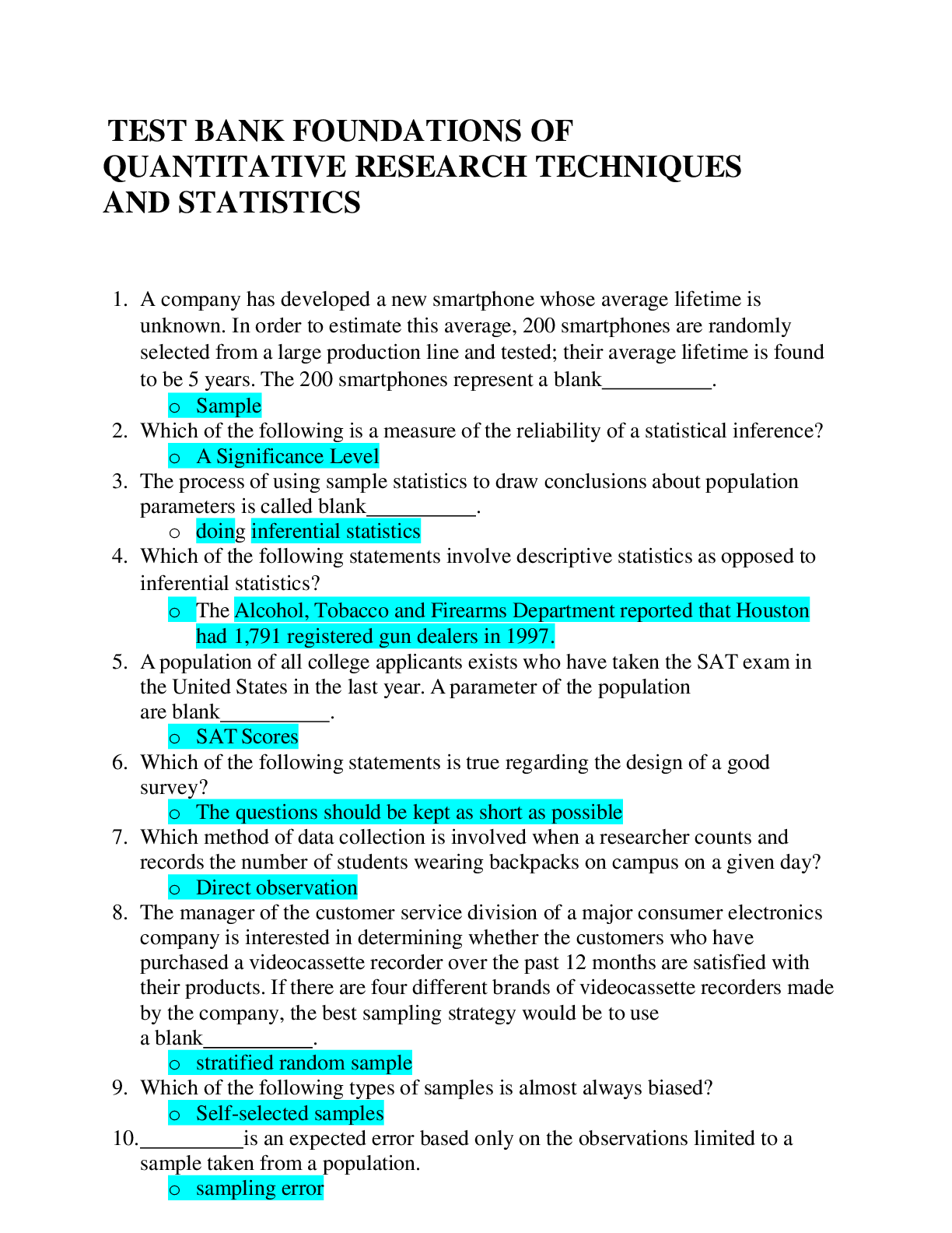
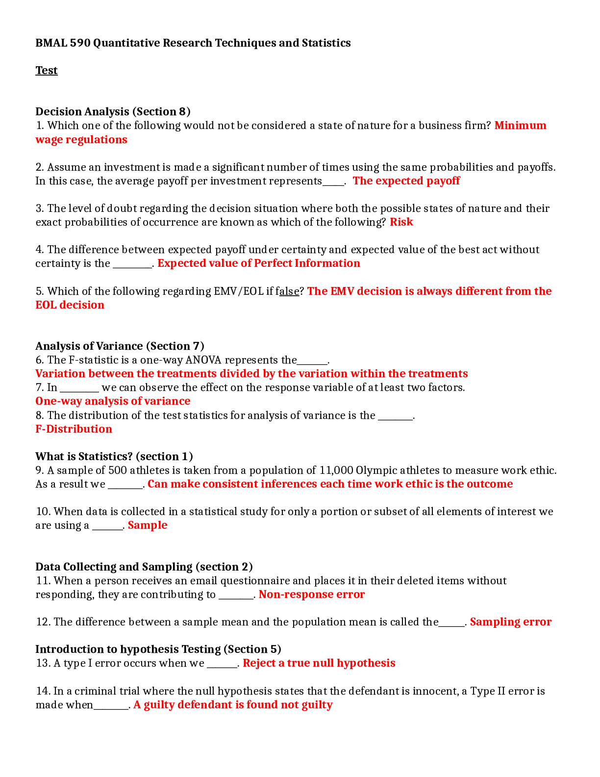
BMAL 590 Quantitative Research Techniques and Statistics BMAL 590 Quantitative Research Techniques and Statistics Test Decision Analysis (Section 8) 1. Which one of the following would not be consider... ed a state of nature for a business firm? 2. Assume an investment is made a significant number of times using the same probabilities and payoffs. In this case, the average payoff per investment represents_____. 3. The level of doubt regarding the decision situation where both the possible states of nature and their exact probabilities of occurrence are known as which of the following? 4. The difference between expected payoff under certainty and expected value of the best act without certainty is the _________. 5. Which of the following regarding EMV/EOL if false? Analysis of Variance (Section 7) 6. The F-statistic is a one-way ANOVA represents the_______. 7. In _________ we can observe the effect on the response variable of at least two factors. 8. The distribution of the test statistics for analysis of variance is the ________. What is Statistics? (section 1) 9. A sample of 500 athletes is taken from a population of 11,000 Olympic athletes to measure work ethic. As a result we ________. 10. When data is collected in a statistical study for only a portion or subset of all elements of interest we are using a _______. Data Collecting and Sampling (section 2) 11. When a person receives an email questionnaire and places it in their deleted items without responding, they are contributing to ________. 12. The difference between a sample mean and the population mean is called the______. Introduction to hypothesis Testing (Section 5) 13. A type I error occurs when we _______. 14. In a criminal trial where the null hypothesis states that the defendant is innocent, a Type II error is made when________. 15. The p-value of the test is the______. Probability (Section 3) 16. Initial estimates of the probabilities of events are known as_____. 17. If the outcome of event A is not affected by event B, then events A and B are said to be ________. 18. The collection of all possible outcomes of an experiment is called ________. 19. Suppose P(A) = .35. The probability of the complement of A is _______. Inference about a Population (Section 6) 20. An unbiased estimator is ________. QUIZ Section 1- A company has developed a new smartphone whose average lifetime is unknown. In order to estimate this average, 200 smartphones are randomly selected from a large production line and tested. Their average lifetime is found to be 5 years. 200 smartphones represents a ________. Which of the following is a measure of reliability of a statistical inference? The process of using sample statistics to draw conclusions about population parameters is called_____. Which of the following statements involve descriptive statistics as opposed to inferential statistics? A population of all college applicants exists who have taken the SAT exam in the US in the last year. A parameter of the population are______. QUIZ Section 2 -Which of the following statements is true regarding the design of a good survey? -Which method of data collection is involved when a researcher counts and records the number of students wearing backpacks on campus in a given day? -Manager at electronics store wants to know if customers who purchased video recorder over the last 12 months are satisfied with their products. If there are 4 different brands of video recorders made by the company, which sampling strategy would be best to use? -Which of the following types of samples are almost always biased? -_____ is an expected error based only on the observations limited to a sample taken from a population. QUIZ Section 3 Bayes’ Law is used to compute ____. The classical approach describes a probability_________. If a set of events includes all possible outcomes of an experiment these events are considered to be________. Which statement is not correct? i QUIZ Section 4- The concept that allows us to draw conclusions about the population based strictly on sample data without having any knowledge about the distribution of the underlying population is_________. The central limit theorem Each of the following are characteristics of the sampling distribution of the mean except________. -Suppose you are given 3 numbers that relate to the number of people in a university sample. The three numbers are 10,20,30. If the standard deviation is 10, the standard error equals___ . You are tasked with finding the standard deviation. You are given 4 numbers. Numbers are 5, 10, 15, and 20. The standard deviation equals. Two methods exist to create a sampling distribution. Once involves using parallel samples from a population and the other is to use the______. QUIZ Section 5 The hypothesis of most interest to the researcher is the______. A Type I error occurs when________. Statisticians can translate p values into several descriptive terms. Suppose you typically reject H0 at a level of .05. Which of the following statements is incorrect? In a criminal trial where the null hypothesis states that the defendant is innocent a type I error is made when________. To take advantage of the information of a test result using the rejection region method and make a better decision on the basis of the amount of statistical evidence we can analyze the _____. Quiz Section 6 An unbiased estimator is ________. Thirty-six months were randomly sampled and the discount rate on new issues of 91-day Treasury Bills was collected. The sample mean is 4.76% and the standard deviation is 171.21. What is the unbiased estimate for the mean of the population? a 98% confidence interval estimate for a population mean is determined to be 75.38 to 86.52. If the confidence level is reduced to 90%, the confidence interval for the population mean ____ Suppose the population of blue whales is 8,000. Researchers are able to garnish a sample of oceanic movements from 100 blue whales from within this population. Thus_____ In the sample proportion, represented by p=x/n the variable x refers to: QUIZ Section 7 Distribution of the test statistic for the analysis of variance is the______. In Fisher’s least significant difference (LSD) multiple comparison method, the LSD value will be the same for all pairs of means if______. One-way ANOVA is applied to 3 independent samples having means 10, 13, and 18 respectively. If each observation in the 3rd sample were increased by 30, the value of the F statistic would______. Assume a null hypothesis is found to be true. By dividing the sum of squares of all observations or SS (Total) by (n-1) we can retrieve the______.Which of the following is true about a one-way analysis of variance? QUIZ section 8 A tabular presentation that shows the outcome for each decision alternative under the various states of nature is called a ______. Which of the following statements is false regarding the expected monetary value (EMV)? In the context of an investment decision, _______ is the difference between what the profit for an act is and the potential profit given an optimal decision. The branches in a decision tree are equivalent to______. Which of the following is not necessary to compute posterior probabilities? Concerning test statistics sum of squares for error measures the ____. The average speed of cars passing a checkpoint is 60 miles per hour with a standard deviation of 8 miles per hoir. Fifty passing cars are clocked at random from this checkpoint. the probability that the sample mean will be between 57 and 62 miles per hour is? Which of the following do not represent an advantage of taking a sample: __________addresses unknown parameters in the real world that parallel descriptive measures of very large populations. A confidence interval is defined as___________. _______ are utilized to make inferences about certain population parameters. if when using the confidence interval estimator of a proportion the researcher finds there is no chance of finding success in the population, adding the number 4 to the sample size could be part of the solution, which refers to ____. A _______ sample involves diving the population into groups then randomly selecting some of the groups and taking either a sample or a census of their members. Suppose we have a test hypothesis at a significance level of .01 where the resulting F-ratio value is 3.2. The degrees of freedom from the numerator are 10 and the denominator are 20. The p-value of the test is .0129 and we can claim the result: assume a null hypothesis is found true. By dividing the sum of squares of all observations or SS(total) by (n-1), we can retrieve the ______. Historically, a company that mails its monthly catalog to potential customers receives orders from 8 percent of the addresses. If 500 addresses are selected randomly from the last mailing, what is the probability that between 35 and 50 orders were received from this sample? Section 1- What is Statistics? What is Statistics? • Statistics is a way to get information from data. It is a tool for creating new understanding from a set of numbers. Descriptive Statistics • Descriptive Statistics- is one of two branches of statistics, which focuses on methods of organizing, summarizing, and presenting data in a convenient and informative way. o One form of descriptive statistics uses graphical techniques, which allow statistics practitioners to present data in ways that make it easy for the reader to extract useful information.  Histogram (bar graph) can show if the data is evenly distributed across the range of values, if it falls symmetrically from a center peak (normal distribution), if there is a peak but more of the data falls to one side (skewed distribution), or if there are two or more peaks in the data (bi-or multi-modal)  Numerical Techniques- rather than providing raw data the professor may only share summary data with the student. One such method used frequently calculates the average or mean • Measure of central location- the mean (average) is one such measure, it is the sum of all data values divided by the number of values • Range- the simplest measure of variability, is calculated by subtracting the smallest number from the largest. • Median- midpoint of the distribution where 50% of the data values are high and 50% are lower. (not that the mean and median will not necessarily be an observed test score). • Mode- the most frequently occurring data value • Variance- the average squared deviation to the mean. To compute the difference between each data value and the mean is calculated and squared. If differences are not squared sum will always be 0. • Standard deviation • - simply the square root of the variance and gets the variability measure back to the same units as the data • Negatively skewed if mean is to the left (point is to the right), positively skewed if the mean is to the right (point is to the left) Inferential Statistics • Inferential statistics is a body of methods used to draw conclusions or inferences about characteristics of population based on sample data o Example of inferential statistics is exit polling during elections o Practitioners can control the fraction of the size of the sample with between 90-99% Key Statistical Concepts • Statistical inference problems involve three concepts: o population- the group of all items of interest to a statistics practitioner. Frequently very large and may in fact be infinitely large. Does not necessarily refer to a group of people  parameter- descriptive measure of a population, represents the information we need o sample – set of data drawn from the population o statistical inference- we use statistics to make inferences about parameters. Statistical inference is the process of making an estimate, prediction, or decision about a population based on sample data.  Build in measure of reliability • Confidence level- proportion of times that an estimating procedure will be correct  Significance level- measures how frequently the conclusion will be wrong in the long run • Statistic- a descriptive measure of a sample • Populations have parameters while samples have statistics • Since Statistical inference involves using statistics to make inferences about parameters, we can make an estimate, prediction or decision about a population based on sample data • Statistical inference only deals with making conclusions about the unknown population parameters based on the observed sample statistics. • Confidence and Significance levels • Confidence level significance level=1 o Example- if confidence level is 95% the significance level is 5% because must equal 1 QUIZ Section 1- A company has developed a new smartphone whose average lifetime is unknown. In order to estimate this average, 200 smartphones are randomly selected from a large production line and tested. Their average lifetime is found to be 5 years. 200 smartphones represents a ________. Which of the following is a measure of reliability of a statistical inference? The process of using sample statistics to draw conclusions about population parameters is called_____. Which of the following statements involve descriptive statistics as opposed to inferential statistics? A population of all college applicants exists who have taken the SAT exam in the US in the last year. A parameter of the population are______. Section 2- Data Collecting and Sampling Methods of collecting data • Statistics is a tool for converting data into information • Number of methods that produce data o Data are the observed values of a variable o We define a variable or variables that are of interest to us and then proceed to collect observations of those variables. • Three popular methods to collect data for statistical analysis- o Direct Observation- ex. Number of customers entering a bank per hour  Simplest method to obtain data  Data said to be observational  Many drawback to direct observation including that it is difficult to produce useful information in a meaningful way  Advantage is low cost o Experiments- ex new ways to produce things to minimize costs  Sample is split into two groups, one who does something and the other does not then evaluate results from two groups o Surveys – one of the most familiar data collecting methods. Solicit information from people concerning such things as their income, family size and opinions on various issues. Majority are conducted for private use.  Response rate- the proportion of all people who were selected to complete the survey • Low response rate- can destroy the validity of any conclusion resulting from statistical analysis. Need to ensure data is reliable.  Personal interview- many researchers believe this is the best way to survey people, involves an interviewer soliciting information from a respondent. Has higher response rate. Main disadvantage is the cost.  Telephone interview- usually less expensive but also les personal and lower expected response rate o Self-administered questionnaire- usually mailed to sample of people. Inexpensive, but usually have low response rate, have high number of incorrect responses due to misunderstanding questions Questionnaire Design • Must be well thought out, key design principles include: o Keep short as possible o Ask short, simple, clearly worded questions, o Start with demographic questions o Use dichotomous (yes/no) and multiple choice for ran o Use open ended questions cautiously o Avoid using leading questions o Try questionnaire to small number of people first to uncover problems o Think about the way you intend to use the collected data when preparing the questionnaire Sampling • Chief motives for examining a sample rather than a population are cost and practicality • Target population – the population about which we want to draw inferences • Sampled population- actual population from which the sample has been taken • Sampled and target populations should be close to one another Simple Random Sampling • Sampling plan is a method or procedure for specifying how a sample will be taken from a population • Three different sampling plans o Simple random Sampling  Sample selected in such a way that every possible sample with the same number of observations is equally likely to be chosen  Ex. Raffle with tickets  Low cost  Can assign numbers to everyone in the population and then randomly select from numbers o Stratified random sampling  Obtained by separating the population into mutually exclusive sets or stata and then drawing simple random samples from each stratum  Ex- gender (male or female), age (number or range) occupation (professional, blue collar, clerical), household income (under $25K, over $100K, etc)  Avoid strata when there is no connection between the survey and strata, ex using religion to determine group for survey on tax increase  Advantage is ability to make inferences within each stratum to compare strata (ex looking at lowest income group favors tax increase or compare highest and lowest income groups to determine whether they differ in support of tax increase)  Stratifications must be done where the strata are mutually exclusive, meaning that each member of the population must be assigned exactly one stratum  After population has been stratified, we use simple random sampling to generate complete sample o Cluster sampling  Simple random sample of groups or clusters of elements versus a simple random sample of individual objects  Useful when it is difficult or costly to develop a complete list of the population members, also useful when population elements are dispersed geographically  Ex- randomly select block within a city to gather data from (rather than getting lists of households to use)  Cluster sampling reduces costs  Increased sampling error, as may have many similarities in those you sample Larger sample size usually means more accurate sample estimates Sampling Error • Two major types of error when sample is taken from a population: sampling error and non-sampling error • Sampling error- refers to the differences between the sample and the population that exists only because of the observation that happened to be selected for the sample. o Error that we expect to occur when we make a statement about a population that is based only on the observation contained in a sample taken from a population o Difference between the true (unknown) value of the population mean and its estimate, the sample mean, is the sampling error. Size of the deviation may be large simply due to bad luck that a particularly unrepresentative samples happened to be selected Non-Sampling Error • Non-sampling error- more serious than sampling error because taking a larger sample wont diminish the size or the possibility of occurrence of this error o Result from mistakes that are made in the acquisition of the data an from the sample observations being selected improperly o Three types of non-sampling errors: o 1-Data Acquisition errors- arise from the recording of incorrect responses. May be result of incorrect measurement taken because of faulty equipment, mistakes made during transcription from primary sources, inaccurate recording of data due to misinterpretation of terms or inaccurate responses to questions concerning sensitive issues o 2- Non-Response Error- refers to error or bias introduced when responses are not obtained from some members of the sample. When this happens sample observations may not be representative of the target population resulting in biased results.  Response rate- the proportion of all people selected who complete the survey, key survey parameter and helps in understanding the validity of the survey and sources of non-response error o 3- Selection bias- occurs when the sampling plan is such that some members of the target population cannot possibly be selected for inclusion in the sample. Together with non-response error selection bias • When responses are not received from a sampled person bias is introduced QUIZ Section 2 -Which of the following statements is true regarding the design of a good survey? -Which method of data collection is involved when a researcher counts and records the umber of students wearing backpacks on campus in a given day? -Manager at electronics store wants to know if customers who purchased video recorder over the last 12 months are satisfied with their products. If there are 4 different brands of video recorders made by the company, which sampling strategy would be best to use? -Which of the following types of samples are almost always biased? -_____ is an expected error based only on the observations limited to a sample taken from a population. Section 3- Probability probability to events • Random experiment- is an action or process that leads to one of several possible outcomes Requirements of Probabilities • Step 1- produce a list of outcomes. List must be exhaustive, meaning all possible outcomes must be included. Outcomes must be mutually exclusive meaning that no two outcomes can occur at the same time o Sample space- list of exhaustive and mutually exclusive outcomes (denoted by S) o S= {O1, O2…..Ok} o Once sample space is prepared we begin the task of assigning probabilities to the outcomes. There are 3 approaches to assign probability to outcomes, each must follow the two rules governing probabilities  1- the probability of any outcome must lie between 0 and 1 • 0<_ P(Oi)<_1  2- The sum of the probabilities of all outcomes in a sample space must be 1 • EKi=1P(Oi)=1 Three approaches to Assigning Probabilities • Classical approach- used by mathematicians to help determine the probability associated with games of chance.  If an experiment has n possible outcomes, this method would assign a probability of 1/n to each outcome. • Ex- toss of coin, sum of probability must be 1, so probability for heads and tails are both ½ or 50%. For dice it is 1/6 • Relative Frequency Approach- defines probability as the long run relative frequency with which an outcome occurs usually as a percentage o Ex. If 200 out of 1000 kids received an A in the class, the relative frequency is 200/1000 or 20%. o This figure is a relative estimate of the probability of obtaining an A • Subjective approach- we define probability as the degree of belief that we hold in the occurrence of an event. Can be described as hunches or educated guesses o Use when it is not reasonable to use the classical approach and there is no history of outcomes for the relative freq. approach. Interpreting Probability • No matter which method is used to assign probability, we interpret it using relative frequency approach for an infinite number of experiments. • Relative frequency approach is useful to interpret probability statements such as those heard from weather forecasters or scientists o This is also the way we link the population and the sample to the statistical inference Joint Probability • How to calculate the probability of more complicated events from the probability of related events. • Intersection of two events is one of the most important ways to look at combinations and relationships between events, ex. A intersects B or A  B • The probability of the intersection is called the Joint probability. • A  B is A union B • Joint probabilities allow us to compute various probabilities Marginal Probability • Marginal Probability is a measure of the likelihood that a particular event will occur regardless of were another event occurs. o Computed by adding across rows or down columns are so named because they are calculated in the margins of the table  Ex. With MBA program grads running successful mutual funds, add top MBA grads and get .40 or 40% of all mutual fund managers graduated from top MBA program. Combination of all must still add to 1, non top mba is .60 or 60% Conditional Probability • Conditional Probability is used to determine how two events are related, that is we can determine the probability of on event given the occurrence of another related event. The probability of an event given that another event has occurred. o Called a conditional probability because we want to know the probability given a certain condition o Ex. Probability that a fund manager by a top MBA grad will outperform the market, given the manager graduated from a top school • Conditional probabilities are written as P(A|B) read as the probability of A given B • Calculation on conditional probabilities raises the question of whether the two events are related Independence • One of the objectives in calculating a conditional probability is to determine if the two events are related. In particular we would like to know if thy are independent events. • Two events are said to be independent if: P(A|B)=P(A) or P(B|A)=P(B) • Independent- two events are independent if the probability of one event is not affected by the occurrence of another event. • Ignore mutually exclusive combinations • In each combination in the example the two events are independent, in this type of problem when one combination is dependent all 4 will be dependent or visa versa. This rule does not play to any other situation. Union • Union is another combination of events, the Union of events A and B is the event that occurs when either A or B or both occur denoted as A  B • Ex. To determine that a randomly selected fund outperforms the market or the manager graduated from a top MBA program, we will need to compute the union of the two events. Union occurs when: o Fund out performs the market and the manager graduated from a top mba program o Fund outperforms the market and the manager did not graduate from a top mba program o Fund does not out perform the market and the manager graduated from a top mba program Complement Rule • Complement of event A is the event that occurs when event A does not occur. Complement of event A is denoted as Ac. Event consisting of all sample points that are “not in A” o The compliment of the rule defined here derives from the fact that the probability of an event and the probability of the events complement must sum to 1 • Compliment rule is P(Ac)=1-P(A) for any event A o Ex. Roll of die, probability the number “1” is rolled is 1/6, the probability that some other number than “1” will be rolled is 1-1/6=5/6 Multiplication Rule • Multiplication rule is used to calculate the join probability of two events. It is based on the formula for conditional probability defined earlier. o P(A|B)=P(A  B)/P(B) o We derive the multiplication symbol my multiplying both sides by P(B) o Joint probability of ay two events is P(A  B)= P(A)xP(B|A) o Ex. Course has 7 male and 3 female students, professor wants to select 2 students at random. o Probability that the 1st student is female- P(A)= 3/10 = .30 o Probability after that event that the second student is female 2/9=.22 o To determine P(A and B)  =(3/10)(2/9) which is =6/90, then = .067 i.e. there is 6.7% chance the professor will choose two female students from the graduate class Multiplication rule for independent events • If A and B are independent events, P(A|B)=P(A) and P(B|A)=P(B), it follows joint probability of two independent events is simply the product of the probability two events • Multiplication rule for independent events- P(A  B)=P(A)xP(B) o Ex. Probability of choosing females to answer questions in classes (if different teachers) is (3/10)=9/10=.09 Addition Rule • Example two newspapers, Sun and Post 22% subscribe to Sun and 3% to post, 6% to both. • P(A  B)= P(A) P(B)- P(A  B) o =.22 .35-.06 o =.51 or 51% probability that the randomly selected household subscribes to one or both newspapers Probability Trees • Effective and simpler way of applying the probability rules is with probability trees, wherein the events in an experiment are represented by lines. Resulting figure resembles a tree • We calculate the joint probabilities by multiplying the probabilities on the linked branches • Probability of selecting two female students for the class is P(F and F)= (3/10) (2/9)=6/90 • At the “ends” of the branches we calculate joint probabilities as the product of the individual probabilities on the preceding branches • Probability tree with replacement- student can be chosen but then chosen again • Advantage of probability trees- restrains users from making the wrong calculation. Once tree is drawn probabilities of branches inserted, virtually the only allowable calculation is the multiplication of the probabilities of linked branches • Check on calculations, joint probabilities at the ends, the branches sum must equal 1, bc all possible events are listed • This special form of the addition rule for mutually exclusive events can be applied to the join probabilities. • No requirement for the branch splits to be binary, nor that the tree only goes two levels deep, or that there be the same number of splits at each sub node Compliment Rule to determine Probability • Example to determine: first time bar test takers have 72% pass rate, if thy fail they can re-take it. Those who fail the first time have an 88% chance they pass on second attempt. • Find the probability that a randomly selected law grad passes. o P(pass[on first exam]) P(fail[on first exam] and pass [on second exam]) o =.72 .2464=.9664 or 96.64% become lawyers by passing first or second exam Bayes’ Law • Conditional probability is often used to gauge the relationship between two events. • In many examples conditional probability measures the probability that an event occurs given that a possible cause of the event has occurred. • Baye’s law is the technique we use to compute the probability of one of the possible causes of a particular event • Ex. Mba applicant is considering gmat prep course • P(A|B)= P(A  B)/P(B) or .052/.259=.201 or that chances are 20.1% when prep course is taken • Prior probabilities because they are determined prior to the decision about taking the preparatory course - P(A) and P(Ac) • Posterior probability (or revised probability) because the prior probability is revised after the decision about taking the prep course – P9A|B) • Bayes’ law can also be expressed in a formula for an algebraic approach Identifying the correct method • Key issue in determining which probability method to use is whether joint probabilities are provided or are required • If joint probabilities are given: o We can compute marginal probabilities by adding across rows or columns o We can use joint and marginal probabilities to compute conditional probabilities for which a formula is available. This allows us to determine whether the events described by the table are independent or dependent. o Can also use the addition rule to compute the probability that either of the two events occurs • If joint probabilities are required (not given): o Need to apply soe or all 3 of the probability rules where one or more joint probabilities are required o Multiplication rule (either by formula or probability tree) to calculate probability of intersections o Addition rule for mutually exclusive events when we want to add the joint probabilities o Compliment rule to determine is an event that occurs when another event does not occur o Bayes’ law to calculate new conditional probabilities • First step in assigning a probability is to create an exhaustive and mutually exclusive list of outcomes. • Second step is to use classical, relative frequency, or subjective approach and assign probability to outcomes. There are very few methods available to compute the probability of other events. These methods include probability rules and trees. An important application of these rules is Bayes’ law which allows us to compute conditional probabilities fro other forms of probability QUIZ Section 3 Bayes’ Law is used to compute ____. The classical approach describes a probability_________. If a set of events includes all possible outcomes of an experiment these events are considered to be________. Which statement is not correct? i Section 4- Sampling Distributions Sampling Distribution of the Mean • Sampling distributions describe the distribution of sample statistics. • A Sampling distribution is created by, sampling. Two ways to create: o 1) Actually draw samples of the same size from a population, calculate the statistic of interest and then use descriptive techniques to learn more about the sampling distribution. o 2) Relies on rules of probability and the laws of expected value and variance to derive the sampling distribution. • Ex looking at 2 dice. Sampling distribution is created by looking at all samples of size n=2 (two dice) and their means • Sampling distribution of the mean has a different mean from the original population • Standard deviation of the sampling distribution mean is referred to as the standard deviation • If the original population is not normally distributed, the sampling distribution of the mean will be normal Standard Error • Sampling error- standard deviation of the sampling distribution o To compute take the standard deviation divided by the square root of the sample size Central Limit Theorem • Variance of the sampling distribution of X is less than the variance of the population were sampling from for all sample sizes o Thus a randomly selected value of X (mean of the umber of spots observed in say 5 throws of dice), is likely to be closer to the mean value of 3.5 than is a randomly selected value X (number of spots observed in one throw) o AS the number of throws increases, probability of the sample mean will also increase o Thus we observe the sampling distribution of X becomes narrower or more concentrated about the mean, as sample size n increases o As n gets larger the sampling distribution of X becomes increasingly bell shaped. • Sampling distribution of the mean of random sample drawn from any population is approximately normal for a sufficiently large sample size. o The larger the sample size the more closely the sampling distribution of X will resemble a normal distribution. • Accuracy of the approximation alluded to in the central limit theorem depends on the probability distribution of the population and on the sample size. Sampling Distribution of the Sample Mean • Statisticians have shown that the mean of the sampling distribution is always equal to the mean of the population and that the standard error is equal to /n for infinitely large populations. If the population is finite, the standard error is • Where N is the population size and N-n/N-1 is called the finite population correction factor. An analysis revealed that if the population size is large relative to the sample size, the finite population correction factor is close to 1 and can be ignored • As a rule of thumb, we treat any population that is at least 20x larger than the sample size as large. • In practice most applications involve populations that qualify as large because if the population is small it may be possible to investigate each member of the population and in doing so calculate the parameters precisely o As a consequence the finite population correlation factor is usually omitted • If x is normal, X (with line) is normal. If X is non-normal, X (with line) is approximately normal for sufficiently large sample sizes. The definition of sufficiently large depends on the extent of non-normality of X. Creating the Sampling Distribution Empirically • To create the sampling distribution empirically, we can actually toss the dice repeatedly, calculating the mean for each sample, counting the number of times each value of X occurs and computing the relative frequencies to estimate the theoretical probabilities. • Disadvantages are excessive amount of time Contents of a 32-oz bottle • Ex. Foreman at a bottling plant observed that the amount of soda in a 32oz bottle is actually normatively distributed random variable, with a mean of 32.2oz and a standard deviation of .3oz o We want to find P(X>32) where X is normally distributed and =32.2 and =.3 o P(Z>.67)=1-.2514=.748 o There is about a 75% chance that a bottle of soda contains more than 32 oz Salaries of business school graduates • We want to fin the probability that the sample mean is less than $750 (earned per week for grad school grads)- P(X<750) • The distribution of X , the weekly income, is likely to be positively skeed but not sufficiently so to make the distribution of X non normal. As a result we may assume that X is normal with the mean x=800 and standard deviation is x=20 • Thus =P(Z<-2.5) or =.5-.4938 which is =.0062 • The probability of observing a sample as low as $750 when the population mean is $800 is extremely small. Because the event is quite unlikely Using the Sampling Distribution for Inference • P(-1.96<Z<1.96)=.95 • The middle 95% of a normal distribution leaves tails of both the left and right of the distribution. The z scores associated with those tails of .025 are - 1.96 Sampling Distribution of a proportion • Proportion of the successes if we are only looking for a yes or no answer. Success is getting the outcome we are interested in even if its broken items. • Binominal experiments because they only have two outcomes (success or failure), and have binomial distribution o The binomial distribution is a Discrete distribution because it can only take on whole number values o The binomial distribution parameter is p, the probability of success in any trial • To compute binomial probabilities we have to assume that p was known. However in the real world, p is unknown, requiring a statistics practitioner to estimate its value from a sample. o Sample proportion is the estimator of a population proportion, that is we count the number of successes in a sample and compute. o P (hat) is where X is the number of successes and n is the sample size. When we can take a sample of size n, were actually conducting a binominal experiment and as such a result, X is binomially distributed. Thus the probability of P(hat) can be calculated from its value of X o Suppose we have a binominal experiment with n=10 and p=.4, To find the probability that the sample proportion P(hat) is less than or equal to .50, we find the probability that X is less than or equal to 5 because 5/10=.50  P(Phat≤.50=P(X≤5)=.8383  We can calculate the probability associated with other values of P(hat) similarly using s binomial distribution calculator or table or computer  Discrete distributions such as the binomial do not lend themselves easily o the kinds of calculation needed for inference. Inference is the reason we need sampling distributions. Fortunately we can approximate the binomial distribution by a normal distribution Normal Approximation to the Binomial Distribution • The normal distribution can be used to approximate a binomial distribution. We developed the destiny function by converting a histogram so that the total area in a rectangle equaled to 1. We can do the same for the binomial distributor. • Ex. X is binomial random variable with n=20 and p=.5. We can easily determine the probability of each value of X where X=0,1,2,3….19,20. Rectangle representing the value of X is drawn so that its area equals the probability. We accomplish this by allowing the height of the rectangle equal the probability and the base of the rectangle equal 1. o If we smooth the rectangles we get a bell shaped curve o Thus to use a normal approximation all we need to do is find the area under the normal curve between 9.5 and 10.5. to find normal probabilities requires us to first standardize by subtracting the mean and dividing the standard deviation. The values for =10 and =2.24 • Normal approximation of the binomial works best when he number of experiments, n(sample size) is large, and the probability of success, p, is close to .5. For the approximation to provide good results two conditions should be met: o 1) np≥ 5 o 2) n(1-p) ≥ 5 o Or both the number of expected successes and expected failures are ≥ 5 • To calculate P(X=10) using the normal distribution, we can find the area under the normal curve between 9.5 and 10.5 o P(X=10) ≈ P(9.5<Y<10.5) Where Y is the normal random variable approximating the binomial random variable X. o P(X=10)=.176 while P(9.5<Y<10.5) = .1742 so the approximation is quite good • Using the laws of expected value and variance, we can determine the mean, variance and standard deviation of P(hat). The standard deviation of P(hat) is called the standard error of the proportion. • P(hat) is approximately normally distributed provided that np and n(1-P) are greater than or equal to 5. Political Survey Example • Politician won 52% votes in election, one year later completing a survey of 300 people to see if they would vote for him again. • The number of respondents who would vote for him is a binomial random variable with n=300 and p=.52. Wee want to determine the probability that the same sample proportion is greater than 50% that is we want to find P(Phat>50) • We know that the sample proportion Phat is approximately normally distributed ith mean np=.52 Sampling distribution of the difference between two means • Another sampling distribution that you will encounter is that of the difference between two sample means. The sampling plan calls for independent random samples drawn from each of two normal populations • The samples are said to be independent if the selection of the members of one sample is independent of the selection of the members of the second sample. o We are interested in sampling distribution of the difference between the two sample means • The central limit theorem states that in repeated sampling from a normal population whose mean is  and whose standard deviation is , the sampling distribution of the sample mean is normal with mean  and the standard deviation of /n • Statisticians have shown the difference between two independent normal random variables is also normally distributed, thus the difference between the two sample means is Xhat1-Xhat2 • if the two populations are not both normally distributed, but the sample sizes are “large” (more than 30), the distribution of Xhat1-Xhat2 is approximately normal • Through the use of laws of expected value and variance, we derive the expected value and variance of the sampling distribution of Xhat1-Xhat2 is normal with mean 1-2 o The standard deviation (which is the standard error of the difference of the two means) o If the populations are non-normal, the sampling distribution is only approximately normal for large sample sizes. The required sample size depends on the extent of non-normality.  However for mot populations, sample sizes of 30 or more are sufficient From here to inference • The primary function of the sampling distribution is statistical inference. Simply put, the knowledge of the population and its parameters allows us to use the probability distribution to make probability statements about individual members of the population. The direction of the arrows indicates the direction of the flow of information. o Probability distribution: population and parameters Probability distribution>individual • We developed the same sampling distribution, wherein knowledge of the parameter and some information about the distribution allow us to make probability statements about a sample statistic. Knowing the population mean and standard deviation and assuming that the population is not extremely non-normal enabled us to calculate a probability statement about a sample mean. o Sampling distribution: population and parameters sampling distribution> statistic • Notice that in applying both probability distributions and sampling distributions, we must know the value of the relevant parameters, a highly unlikely circumstance. In the real world, parameters are almost always unknown because they represent descriptive measurements about extremely large populations. o Statistical inference addresses this problem, it does so by reversing the direction of the flow of knowledge. o We will assume that most population parameters are unknown. The statistics practitioner will sample from the population and compute the required statistic. The sampling distribution of the statistic will enable us to draw inferences about the parameter  Sampling Distribution in inference: statistic Sampling distribution> parameter  The sampling distribution of a statistic is created by repeated sampling form one population. We introduced the sampling distribution of the mean, the proportion, and the difference between the two means. We described how these distributions are created theoretically and empirically. QUIZ Section 4- The concept that allows us to draw conclusions about the population based strictly on sample data without having any knowledge about the distribution of the underlying population is_________. The central limit theorem Each of the following are characteristics of the sampling distribution of the mean except________. -Suppose you are given 3 numbers that relate to the number of people in a university sample. The three numbers are 10,20,30. If the standard deviation is 10, the standard error equals___ . You are tasked with finding the standard deviation. You are given 4 numbers. Numbers are 5, 10, 15, and 20. The standard deviation equals. Two methods exist to create a sampling distribution. Once involves using parallel samples from a population and the other is to use the______. Section 5 Introduction to hypothesis testing Concepts of Hypothesis testing • There are a variety of non statistical applications of hypothesis testing for example criminal trial. • IN a trial, the jury conducts a test of hypothesis, there are two hypothesis tested o Null hypothesis- represented by H0 (H-nought- british for zero), it is H0 if the defendant is innocent o Alternative or research hypothesis and is denoted by H1, in a criminal trial it is H1 if the defendant is guilty. • The hypothesis of most interest to the researcher is the alternative hypothesis • There are only two possible decisions for the jury, convict or acquit the defendant • In statistical parlance, convicting the defendant is equivalent to rejecting the null hypothesis in favor of the alternative (i.e. the jury saying there was enough evidence to conclude the defendant was guilty) • Acquitting the defendant is phrased as not rejecting the null hypothesis in favor of the alternative, which means the jury decided there was not enough evidence to conclude that the defendant was guilty. o Notice we do not say we accept the null hypothesis (in criminal trial this would be interpreted as finding the defendant innocent) Type I and Type II error • There are two possible errors o Type I error- occurs when we reject the true null hypothesis  In criminal trial made when innocent person is wrongly convicted  Probability of denoted by  also called the significance level o Type II error is defined as not rejecting a false null hypothesis  Guilty person is acquitted  Probability of denoted by  (beta) o Error probabilities of  and are  inversely related , meaning an attempt to reduce one will increase another o In our justice system type I errors are regarded as more serious. So the probability of a type I error is small  This is arranged by maintaining the burden of proof on the prosecution (prosecution must prove guilt, defense need not prove anything)  Consequence is the probability of acquitting guilty people is large Critical Concepts in Hypothesis Testing • Five critical concepts in hypothesis testing o 1) there are 2 hypothesis: null and alternative/research hypothesis o 2) testing procedure begins with the assumption that the null hypothesis is true o 3) goal of the process is to determine whether there is enough evidence to infer that the alternative hypothesis is true o 4) there are two possible decisions:  conclude that there is enough evidence to support the alternative hypothesis  conclude that there is not enough evidence to support the alternative hypothesis o 5) two possible errors can be made in any test.  A type 1 error occurs when we reject a true null hypothesis • P(Type I error)=   A type II error occurs when we don’t reject a false null hypothesis (ie accept but don’t say that) • P(Type II error)=  Critical concepts in Hypothesis testing: Concept 1 - The null hypothesis H0 will always state that the parameter equals the value specified in the alternative hypothesis H1 • Example- computer company wants to look at inventory levels at outside warehouses • Manager wants to know whether the mean is different from 350 units • Test hypothesis is H0:  = 350 • Research hypothesis is H1:  ≠ 350 • Testing begins with assuming the null hypothesis is true, until we have further statistical evidence we will assume. Ie we assume H0:  = 350 is true • Goal of the process is to determine whether there is enough evidence to infer that the alternative hypothesis is true.. Is there statistical evidence to determine if this statement is true? H1:  ≠ 350 which is what we are interested to know. • There are 2 possible decisions that can be made: o Conclude that there is enough evidence to support the alternative hypothesis (also stated as rejecting the null hypothesis in favor of the alternative) o Conclude that there is not enough evidence to support the alternative hypothesis (also stated as not rejecting the null hypothesis in favor of the alternative)  Note we DO NOT say we accept the null hypothesis (although this is what it means we are doing) • Once the null and alternative hypothesis are stated, the next step is to randomly sample the population and calculate the test statistic (in this example the sample mean) • If the test statistic value is inconsistent with the null hypothesis, we reject the null hypothesis and infer the alternative hypothesis is true. • For example if we are trying to decide if the mean is not equal to 350, a large value of x, say 600, would provide enough evidence. If x is close to 350 say 355, we could not say that this provides a great deal of evidence to infer that the population mean is different that 350 • Two possible errors can be made in any test: o Type I error occurs when we reject a true null hypothesis o Type II error occurs when we don’t reject a false null hypothesis • P(Type I error)=   Probability of denoted by  also called the significance level • P(Type II error)=  Types of errors • Type I error occurs when we reject a true null hypothesis o Reject H0 when it is true • Type II error occurs when we don’t reject a false null hypothesis o Do not reject H0 when it is false Testing the population mean when the population standard deviation is know • Example- department store manager is considering new billing system. After financial analysis she determines that the new system will be cost effective only if the mean monthly account is more than $170 • Random sample of 400 monthly accounts is drawn, sample mean is $170 • Knows accounts are approximately normally distributed with standard deviation of $65 • can the manager conclude from this that the new system will be cost effective? • To conclude that the system will be cost effective requires the manager to show that the mean account for the customers is greater than $170 o Consequently we set up the alternative hypothesis to express H1:  >170 (install new system)  If the mean is less than or equal to 170 the system will not be cost effective o The null hypothesis is expressed as H0:  ≤ 170 (do not install new system) • We will actually test =170, which is how we specify the null hypothesis: H0:  = 170 o Is a sample mean of 178 sufficiently greater than 170 to allow us to infer that the population mean is greater than 170? Rejection Region method • Two ways to answer the above question: o 1) rejection region method which can be used in conjunction with the computer, but is mandatory for those computing statistics manually o 2) p-value approach, which generally can be employed only in conjunction with a computer and statistical software • Rejection Region method o To make decision about close sample mean o Range of values such that if the test statistic falls into the range, we decide to reject the null hypothesis in favor of the alternative. o Produces a yes or no response to the question: “is there sufficient statistical evidence to infer that the alternative hypothesis is true?”  Implication is that the result of the test will be converted automatically into one of two possible courses of action: • 1- action as result of rejecting the null hypothesis in favor of the alternative, • 2- result of not rejecting the null hypothesis in favor of the alternative. Rejection of the null hypothesis • seems to imply the new billing system will be installed. P Value of a test • Several drawbacks to the rejection region method, foremost the type of information provided by the result of the test. • P value provides what is needed to take full advantage of the information available from the test result and make much better decision to the amount of statistical evidence supporting the alternative hypothesis so that it can be weighed in relation to the other factors, especially financial ones. Interpreting the P value • To properly interpret results of an inferential procedure, must remember that the technique is based on the sampling distribution • Sampling distribution allows us to make probability statements about a sample statistic assuming knowledge of the population parameter o For the example above, the probability of observing a sample mean at least as large as 178 from a population whose mean is 170 is .0069 which is very small. In other words an unlikely event, so we seriously doubt the null hypothesis is true. Consequently we have a reason to reject the null hypothesis and support the alternative. o We cannot make a probability statement about a parameter as it is not a random variable/ • P value of a test provides valuable information because it measures the amount of statistical evidence that supports the alternative hypothesis. • The smaller the p value the more statistical evidence supports the alternative hypothesis Describing the P Value • How small does the p value have to be to infer that the alternative hypothesis is true? o Answer depends on the number of factors including costs of making type I and type II errors. o Type I error would occur if the manager adopts the new billing system when it is not cost effective. If cost error is high we would attempt to minimize its probability  Rejection region method, we would do this by setting the significance level quite low say 1%  P value method we would insist the p value be quite small, providing sufficient evidence to infer that the mean monthly account is greater than $170 before proceeding with new billing system. • Statistics practitioners can translate p values using the following descriptive terms: if the p value is less than .01 there is overwhelming evidence to infer that the alternative hypothesis is true. The test is highly significant. o If the p value lies between .01 and .05 there is strong evidence to infer that the alternative hypothesis is true. The result is deemed to be significant o If the p value is between .05-.10 there is weak evidence to indicate that the alternative o hypothesis is true. Over .1 no evidence. The P Value and rejection region methods • We can choose to use the p value to make the same type of decisions we make with the rejection region method • Rejection region method requires the decision maker to select a significance level from which the rejection region is constructed • We then decide to reject or not reject the null hypothesis • Another way of making the decision is to compare the –value with the selected value of significance level • If the p value is less than  we judge the p value to be small enough to reject the null hypothesis. If the p value is greater then  we do not reject the null hypothesis. o Since P value=.0069<=.05 we reject H0 in favor or H1 • Use p value when computer is available, use rejection region when computing manually Interpreting the results of a test • In our example we rejected the null hypothesis. This does not prove that the alternative hypothesis is true because our conclusion is based on sample data, not the entire population. We can never prove anything by using statistical inference. • We summarize the test by saying “there is enough statistical evidence to infer that the null hypothesis is false and that the alternative hypothesis is true” • If the value does not fall into the rejection region ( p value is too large) rather we say we accept the null hypothesis, we say we do not reject the null hypothesis and we conclude that not enough evidence exists to show that the alternative hypothesis is true. • The conclusion is based on the alternative hypothesis. o If we reject the null hypothesis we conclude there is enough statistical evidence to infer that the alternative hypothesis is true o If we do not reject the null hypothesis we conclude there is not enough statistical evidence to infer that the alternative hypothesis is true • Alternative hypothesis is focus in conclusion, it represents what we are investigating o Why it is called a research hypothesis o You have 3 choices for alternative hypothesis the parameter is greater than, less than or not equal to the value specified in the null hypothesis. SSA Envelope Plan • Fed ex wants to improve their payment withing30 days. Current mean is 24 and standard deviation is 6 days. CFO thinks included stamped envelope will improve cash flow by a 2-day increase in payment period. • Objective is to draw a conclusion about the mean payment period. Parameter tested is the population mean. We want to know if there is enough statistical evidence to show the population mean I less than 22 days. o Alternative hypothesis is H1:  < 22 o Null Hypothesis is H0;  = 22 • To solve manually we need to define the rejection region which requires us to specify a significance level. 10% is significance level deemed to be appropriate. • We wish to reject the null hypothesis in favor of the alternative only if the sample mean and hence the value of the test statistic is small enough. o As a result we locate the rejection region in the left tail of the sampling distribution o Remember we are trying to determine if there is enough statistical evidence to infer the mean is less than 22 ( alternative hypothesis) o If we observe a large sample mean ( hence a large value of z) do we want to reject the null hypothesis in favor of the alternative? NO.  It is illogical to think that if the sample mean is say 30 that there is enough evidence to conclude that the mean payment for all customers would be less than 22.  We want to reject the null hypothesis only if the sample mean ( and value of test statistic z) is small. Which is determined by the significance level and rejecton region.  Direction of inequality in the rejection region matched the direction of inequality in the alternative hypothesis. o Value of test statistic is -.91 and p value is .181 which does not allow us to reject the null hypothesis o Because we were not able to reject the null hypothesis we say there is not enough evidence to infer that the mean payment period is less than 22 days One tail test • The rejection region is located in only one tail of the sampling distribution • Right tail test – right side positive Two tail test • Two tail testing is used when we want to test a research hypothesis that a parameter is not equal to some value AT&T Example • Scenario: several companies have formed that offer competition against AT&T for long distance calls. Al advertise their rates are lower than AT&T, resulting in lower bills • AT&T responded arguing customers will see no difference in billing o Statistics practitioner for AT&T determined that mean is $17.09 and standard deviation is $3.87 o He takes 100 customers and recalculates their last month bills using rates quoted by leading competitors. o Assuming the same standard deviation of this population can we conclude at the 5% significance level that there is no difference between the average AT&T bill and the one of the leading competitor? o In this problem we want to know whether the mean monthly long distance bill is different from $17.09. o Consequently we set up the alternative hypothesis to express this condition H1:  ≠ 17.09 o So the null hypothesis is H0:  = 17.09 o Rejection region (left small tail or right small tail) is set up so we can reject the null hypothesis when the test statistic is large or when it is small  Total area in the rejection region must sum to a , so we divide this probability by 2  At a 5% significance level (i.e. =.05), we have a /2 =.025 thus z.025 =1.96  Z<-1.96 or z>1.96 o Since z=1.19 is not great than 1.96 or less than -1.96 we cannot reject the null hypothesis in favor of H1. That is there is insufficient evidence to infer that there is a difference between the bills • We can also compute the p value of the test. Because it is a 2-ailed test, we determine the p value by finding the area in both tails o The p value= P(Z<-1.96 P(>1.19)= .1170 .1170=.2340 o Or more simply multiple the probability in one tail by 2. In general the p value in a 2 tail test is determined by p value=2P(Z>|z|) where z is the actual value of the statistic and |z| is its absolute value o There is not enough evidence to infer that the mean long distance bill is different from AT&Ts mean of $17.09 When do we conduct two tail tests • A two tail test is conducted whenever the alternative hypothesis specifies that the mean is not equal to the value stated in the null hypothesis, that is when the hypothesis assume the following form o H0:  = 0 o H1:  ≠ 0 • There are two one-tail tests. We conduct a one tail test focused on the right tail of the sampling distribution whenever we want to know whether there is enough evidence to infer that the mean is greater than the quantity specified in the null hypothesis, that is when our hypothesis are: o H0:  = 0 o H1:  > 0 • The second one tail test involves the left tail of the sampling distribution. It is used when the statistics practitioner wants to determine whether there is enough evidence to infer that the mean is less than the value of the mean stated in the null hypothesis o H0:  = 0 o H1:  < 0 Testing Hypothesis and Confidence Interval Estimators • The test statistic and confidence internal estimator are both derived from the sampling distribution • We can use the confidence interval estimator to test hypothesis • LCL- lower confidence limit • UCL- Upper confidence limit • LCL- 16.79 and UCL is 18.31 • Because $17.09 lies between we cannot conclude that there is sufficient evidence to infer that the population mean differs from 17.09 • For the department store billing example, the 95% confidence level interval estimate is LCL=171.63 and UCL 184.37 o Since the interval estimate includes 170 allowing us to conclude that the population mean account is not equal to $170 • The confidence interval estimator can be used to conduct tests of hypothesis • This process is equivalent to the rejection region approach, however instead of finding the critical values of the rejection region and determining whether the test statistic falls into the rejection region, we compute the interval estimate and determine whether the hypothesizes value of the mean falls into the interval Advantage • Interval estimator to test hypothesis has the advantage of simplicity. Apparently we don’t need a formula for the test statistic we need only the interval estimator Disadvantage • When conducting a one tail test or conclusion may not answer the original question o Example in the department store billing example, we wanted to know whether there was enough evidence to infer that the mean is greater than 170. The estimate concludes the mean differ from 170. In attempting to draw the conclusion that the entire interval is greater than 170 there is enough statistical evidence to infer the population mean is greater than 170, however we run into the problem of determining the procedures significance level. Is it [Show More]

Last updated: 1 year ago

Preview 1 out of 49 pages