Concordia UniversityMECH 412412_Assignment_3_2008F_solution Computer Aided Mechanical Design

Document Content and Description Below

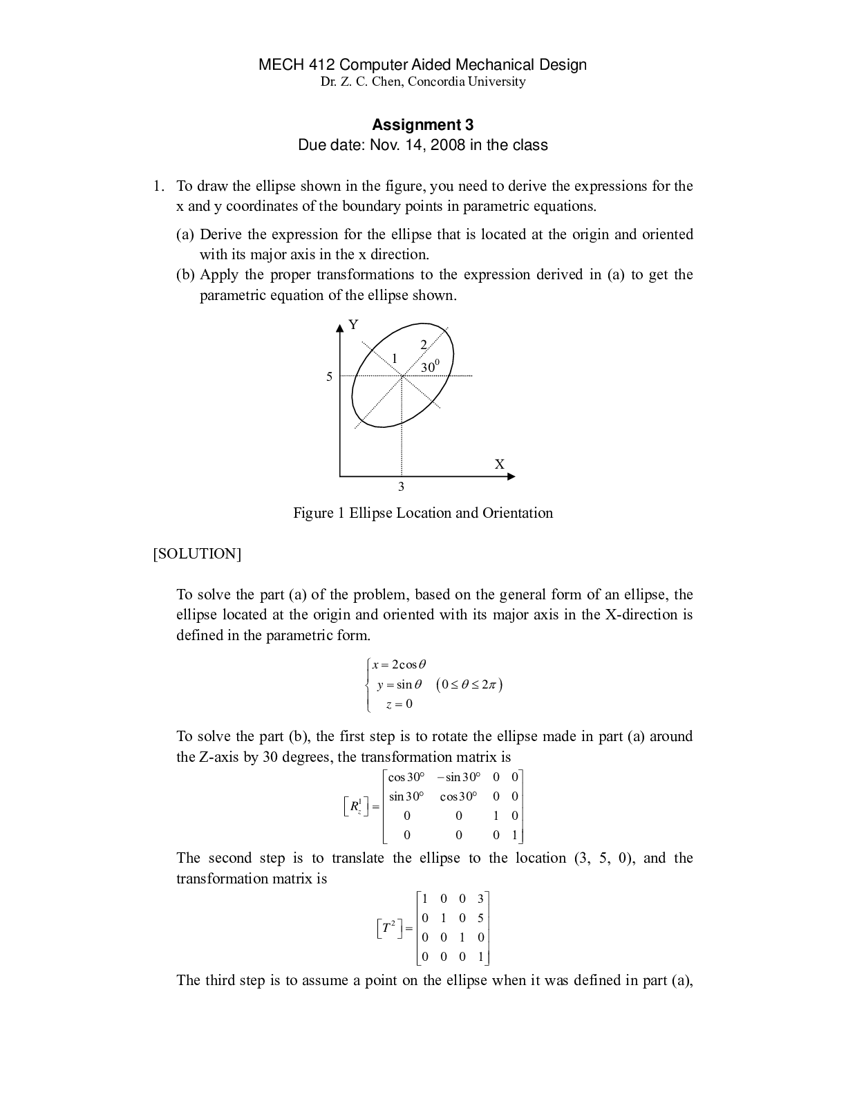
MECH 412 Computer Aided Mechanical Design Dr. Z. C. Chen, Concordia University Assignment 3 Due date: Nov. 14, 2008 in the class 1. To draw the ellipse shown in the figure, you need to derive the ... expressions for the x and y coordinates of the boundary points in parametric equations. (a) Derive the expression for the ellipse that is located at the origin and oriented with its major axis in the x direction. (b) Apply the proper transformations to the expression derived in (a) to get the parametric equation of the ellipse shown. Figure 1 Ellipse Location and Orientation [SOLUTION] To solve the part (a) of the problem, based on the general form of an ellipse, the ellipse located at the origin and oriented with its major axis in the X-direction is defined in the parametric form. ( ) 2cos sin 0 2 0 x y z θ θ θ π ⎧ = ⎪ ⎨ = ≤ ≤ ⎪ ⎩ = To solve the part (b), the first step is to rotate the ellipse made in part (a) around the Z-axis by 30 degrees, the transformation matrix is 1 cos30 sin 30 0 0 sin 30 cos30 0 0 0 0 1 0 0 0 0 1 Rz ⎡ ° − ° ⎤ ⎢ ⎥ ⎡ ⎤ ⎣ ⎦ = ⎢ ⎢ ° ° ⎥ ⎥ ⎢ ⎥ ⎢ ⎣ ⎥ ⎦ The second step is to translate the ellipse to the location (3, 5, 0), and the transformation matrix is 2 1 0 0 3 0 1 0 5 0 0 1 0 0 0 0 1 T ⎡ ⎤ ⎢ ⎥ ⎡ ⎤ ⎣ ⎦ = ⎢ ⎢ ⎥ ⎥ ⎢ ⎥ ⎢ ⎣ ⎥ ⎦ The third step is to assume a point on the ellipse when it was defined in part (a), 3 5 2 1 300 X YMECH 412 Computer Aided Mechanical Design Dr. Z. C. Chen, Concordia University the coordinate of the point at the new location is calculated as 3 1 2 2 1 3 2 2 1 0 0 3 cos30 sin 30 0 0 3 0 1 0 5 sin 30 cos30 0 0 5 0 0 1 0 0 0 1 0 1 0 0 0 1 0 0 0 1 1 1 x x x y y y x y z z z ⎡ ⎤ ⎡ ⎤ ⎡ ⎤ ⎡ ⎤ ′ ° − ° − + ⎡ ⎤ ⎢ ⎥ ⎢ ⎥ ⎢ ⎥ ⎢ ⎥ ⎢ ⎥ ⎢ ⎥ ⎢ ⎥ ⎢ ⎥ ′ = = ° ° ⎢ ⎢ + + ⎥ ⎥ ⎢ ⎥ ⎢ ⎥ ⎢ ⎥ ⎢ ⎥ ′ ⎢ ⎥ ⎢ ⎥ ⎢ ⎥ ⎢ ⎥ ⎢ ⎥ ⎢ ⎥ ⎢ ⎥ ⎢ ⎥ ⎢ ⎥ ⎢ ⎥ ⎣ ⎦ ⎣ ⎦ ⎣ ⎦ ⎣ ⎦ ⎢ ⎣ ⎥ ⎦ Thus the parametric form of the ellipse is ( ) 12 3 2 3 cos sin 3 cos sin 5 0 2 0 x y z θ θ θ θ θ π ⎧ ′ = − + ⎪ ⎪ ⎨ ′ = + + ≤ ≤ ⎪ ′ = ⎪ ⎩ [END] 2. Consider a Hermite curve on the xy plane defined by the following geometric coefficients: (0) 2 3 (1) 4 0 (0) 3 2 3 4 (1) p p p p ⎡ ⎤ ⎡ ⎤ ⎢ ⎥ ⎢ ⎥ ⎢ ⎥ ⎢ ⎥ ⎢ ⎥ ′ = ⎢ ⎥ ⎢ ⎥ ⎢ ⎥ ⎢ ⎥ ⎣ ⎦ ′ ⎢ ⎥ ⎣ ⎦ − JG JG JJG JJG (a) Find a Bezier curve of degree 3 to represent the given Hermite curve as exactly as possible. In other words, determine the four control points of the Bezier curve. (b) Expand both of the curve equations in polynomial form and compare them. [SOLUTION] To find a Bezier curve of degree 3 to approximate the given Hermite curve in part (a), the four control points of the Bezier curve should be determined. One of the properties of Bezier curves is the curve passes through the first and last control points. Thus the two ends of the Hermite curve are the first and last control points, respectively. 0 3 ( ) 0 , (1) 2 4 3 0 P p P p = = = = ⎡ ⎢ ⎤ ⎡ ⎤ ⎥ ⎢ ⎥ ⎣ ⎦ ⎣ ⎦ JG JG The first-order derivative of a Bezier curve is provided in the textbook. 1 1 ( ) 1 0 ( ) 1 (1 ) n i n i i i i d p u n n u u P P du i − − − + ∑= ⎛ ⎞ − = ⋅ ⋅ − ⋅ − ⎜ ⎟ ⎝ ⎠ JG When u is equal to zero, 1 0 0 ( ) ( ) u d p u n P P du = = − JG ; when u is equal to one,MECH 412 Computer Aided Mechanical Design Dr. Z. C. Chen, Concordia University 3 2 1 ( ) ( ) u d p u n P P du = = − JG . The tangent vectors of the Hermite curve at the ends are also given. The other two control points ( P P 1 2 , ) can be found with the following equations. ( ) ( ) 0 1 ( ) ' 0 ( ) ' 1 u u d p u p du d p u p du = = = = JG JG JG JG Solving the two equations, the control points, P P 1 2 , , can be calculated. 1 2 11 4 3 3 3 3 P P , ⎡ ⎤ ⎡ ⎤ = = ⎢ ⎥ ⎢ ⎥ ⎣ ⎦ ⎣ ⎦ After the four control points are found, the Bezier curve is expressed as 0 , 0 3 1 2 2 2 1 3 3 0 0 1 2 3 2 3 2 3 2 3 3 0 1 2 3 2 3 2 3 11 ( ) ( ) 3 3 3 3 (1 ) (1 ) (1 ) (1 ) 0 1 2 3 (1 3 3 ) (3 6 3 ) (3 3 ) 2 3 (1 3 3 ) (3 6 3 ) 3 n i i n i P u P B u u u P u u P u u P u u P u u u P u u u P u u P u P u u u u u u ∑= = ⋅ ⎡ ⎤ ⎡ ⎤ ⎡ ⎤ ⎡ ⎤ = ⋅ ⋅ − ⋅ + ⋅ ⋅ − ⋅ + ⋅ ⋅ − ⋅ + ⋅ ⋅ − ⋅ ⎢ ⎥ ⎢ ⎥ ⎢ ⎥ ⎢ ⎥ ⎣ ⎦ ⎣ ⎦ ⎣ ⎦ ⎣ ⎦ = − + − ⋅ + − + ⋅ + − ⋅ + ⋅ ⎡ ⎤ = − + − + − + ⎢ ⎥ ⎣ ⎦ ( ) 2 3 3 4 3 3 2 3 2 3 3 4 (3 3 ) 0 2 3 3 2 3 2 9 4 0 u 1 0 u u u u u u u u u ⎡ ⎤ ⎡ ⎤ ⎡ ⎤ ⎢ ⎥ ⎢ ⎥ + − + ⎢ ⎥ ⎣ ⎦ ⎣ ⎦ ⎣ ⎦ ⎡ ⎤ + − + ⎢ ⎥ = + − + ≤ ≤ ⎢ ⎥ ⎢ ⎥ ⎣ ⎦ In part (b) of the question, since the Hermite curve was found before, the equation of the Hermite curve is 2 3 2 3 2 3 2 3 2 3 2 3 2 3 2 3 3 2 3 2 (0) (1) ( ) 1 3 2 3 2 2 (0) (1) (1 3 2 ) (0) (3 2 ) (1) ( 2 ) '(0) ( ) '(1) 2 3 3 2 (0 1) 4 9 2 3 p p p u u u u u u u u u u p p u u p u u p u u u p u u p u u u u u u u ⎡ ⎤ ⎢ ⎥ ⎢ ⎥ = − + − − + − + ⎡ ⎤ ⎣ ⎦ ⎢ ⎥ ⎢ ⎥ ′ ⎢ ⎥ ⎣ ⎦ ′ = − + ⋅ + − ⋅ + − + ⋅ + − + ⋅ ⎡ ⎤ − + + = ≤ ≤ ⎢ ⎥ ⎣ ⎦ − + + JG JG JG JJG JJG JG JG JG JG Comparing the expressions of the Hermite and Bezier curves, the two curves are the same. 3. A Bezier curve defined by the control points A A A 0 1 2 , , and is to be transformed toMECH 412 Computer Aided Mechanical Design Dr. Z. C. Chen, Concordia University the Bezier curve defined by B B B 0 1 2 , , and shown in the following figure. The transformation should move point A B 0 0 to and A B 2 2 to . This means that scaling is also required. (a) Explain which transformation matrices are applied and in which order. (b) Calculate the coordinates of control point B1 . (c) Derive the parametric equation of the resulting curve C2. [SOLUTION] In part (a), to move point A B 0 0 to and A B 2 2 to , first translate the A A 0 2 from the location A0 to the origin. The transformation matrix is 1 1 0 1 0 1 1 0 0 1 T ⎡ − ⎤ ⎡ ⎤ ⎣ ⎦ = ⎢ ⎢ − ⎥ ⎥ ⎢ ⎣ ⎥ ⎦ The angle between B B 0 2 and the X direction is 1 tan ( ) 40.89 1 0 2 3 2 7 5 γ − + − = = − , and the angle between A A 0 2 and the X direction is 2 tan ( ) 45 1 0 4 1 4 1 γ − − = = − . Thus rotate A A 0 2 about the origin by − − 4.11 40.89 45 D D D ( ). The rotation matrix is 2 cos( 4.11 ) sin( 4.11 ) 0 sin( 4.11 ) cos( 4.11 ) 0 0 0 1 R ⎡ − − − ⎤ ⎢ ⎥ ⎡ ⎤ ⎣ ⎦ = − − ⎢ ⎥ ⎢ ⎥ ⎣ ⎦ D D D D The module of A A 0 2 is (4 1) (4 1) 3 2 − + − = 2 2 and the module of B B 0 2 is (7 5) (2 3 2) 7 − + + − = 2 2 . The ratio of the modules is 7 7 S S S = = = = x y 3 2 18 So the scaling matrix is 7 18 3 7 18 0 0 0 0 0 0 0 0 0 0 1 0 0 1 x y S S S ⎡ ⎤ ⎡ ⎤ ⎢ ⎥ ⎡ ⎤ ⎣ ⎦ = = ⎢ ⎥ ⎢ ⎥ ⎢ ⎢ ⎥ ⎥ ⎢ ⎥ ⎣ ⎦ ⎢ ⎥ ⎢ ⎣ ⎥ ⎦ The last step is to translate the point A0 from the origin to the location B0 . The translation matrix isMECH 412 Computer Aided Mechanical Design Dr. Z. C. Chen, Concordia University 4 1 0 5 0 1 2 0 0 1 T ⎡ ⎤ ⎡ ⎤ ⎣ ⎦ = ⎢ ⎢ ⎥ ⎥ ⎢ ⎣ ⎥ ⎦ The equivalent matrix is calculated as [ ] 4 3 2 1 7 18 7 18 0 0 1 0 5 cos( 4.11 ) sin( 4.11 ) 0 1 0 1 0 1 2 0 0 sin( 4.11 ) cos( 4.11 ) 0 0 1 1 0 0 1 0 0 1 0 0 1 0 0 1 0.622 0.045 4.333 0.045 0.622 1.423 0 0 1 E T S R T = ⎡ ⎤ ⎡ ⎤ ⎡ ⎤ ⎡ ⎤ ⎣ ⎦ ⎣ ⎦ ⎣ ⎦ ⎣ ⎦ ⎡ ⎤ ⎡ ⎤ ⎡ ⎤ ⎢ ⎥ ⎡ ⎤ − − − − = − − − ⎢ ⎥ ⎢ ⎥ ⎢ ⎥ ⎢ ⎥ ⎢ ⎥ ⎢ ⎥ ⎢ ⎥ ⎢ ⎥ ⎢ ⎥ ⎢ ⎥ ⎣ ⎦ ⎣ ⎦ ⎢ ⎥ ⎢ ⎥ ⎣ ⎦ ⎢ ⎥ ⎣ ⎦ ⎡ ⎤ ⎢ ⎥ = − ⎢ ⎥ ⎢ ⎥ ⎣ ⎦ D D D D To calculate the coordinate of the location B1 in the part (b) of the problem, apply the equivalent matrix [E] on the problem. The coordinate can be calculated as 1 1 [ ] 0.622 0.045 4.333 2 5.71 0.045 0.622 1.423 3 3.19 0 0 1 1 1 B E A ⎡ ⎤ ⎡ ⎤ ⎡ ⎤ ⎢ ⎥ ⎢ ⎥ ⎢ ⎥ = = − = ⎢ ⎥ ⎢ ⎥ ⎢ ⎥ ⎢ ⎣ ⎥ ⎢ ⎥ ⎢ ⎥ ⎦ ⎣ ⎦ ⎣ ⎦ In part (c) to derive the parametric equation of the resulting curve C2, the three control points are 0 1 2 5 5.71 7 , , and 2 3.19 2 3 B B B ⎡ ⎤ ⎡ ⎤ ⎡ ⎤ = = = ⎢ ⎥ ⎢ ⎥ ⎢ ⎥ ⎣ ⎦ ⎣ ⎦ ⎣ + ⎦ The form of the Bezier curve isMECH 412 Computer Aided Mechanical Design Dr. Z. C. Chen, Concordia University 2 0 2 1 2 0 , 0 1 2 0 0 2 1 2 0 0 1 2 2 2 2 0 1 2 2 2 2 2 ( ) ( ) (1 ) (1 ) (1 ) 0 1 2 2! 2! 2! (1 ) (1 ) (1 ) 0!(2 0)! 1!(2 1)! 2!(2 2)! (1 ) (2 2 ) 5 (1 ) 2 0 i i n i p u B B u u u B u u B u u B u u B u u B u u B u B u u B u B u ∑= ⎡ ⎤ ⎡ ⎤ ⎡ ⎤ = ⋅ = ⋅ ⋅ − ⋅ + ⋅ ⋅ − ⋅ + ⋅ ⋅ − ⋅ ⎢ ⎥ ⎢ ⎥ ⎢ ⎥ ⎣ ⎦ ⎣ ⎦ ⎣ ⎦ = ⋅ ⋅ − ⋅ + ⋅ ⋅ − ⋅ + ⋅ ⋅ − ⋅ − − − = − ⋅ + − ⋅ + ⋅ ⎡⎢ = − ⎢ ⎣ JG 2 2 2 2 5.71 7 (2 2 ) 3.19 3.73 0 0 5 1.42 0.58 2 2.38 0.65 0 u u u u u u u ⎤ ⎡ ⎤ ⎡ ⎤ ⎥ ⎢ ⎥ ⎢ ⎥ ⎥ ⎢ ⎥ ⎢ ⎥ + − + ⎢ ⎥ ⎢ ⎥ ⎢ ⎥ ⎦ ⎣ ⎦ ⎣ ⎦ ⎡ ⎤ + ⋅ + ⋅ ⎢ ⎥ = + ⋅ − ⋅ ⎢ ⎥ ⎢ ⎥ ⎣ ⎦ 4. Determine a Bezier curve of degree 3 that approximates a quarter circle centered at (0, 0). The end points of the quarter circle are (1, 0) and (0, 1). Calculate the coordinates of the middle point of this Bezier curve and compare them with those of the midpoint of the quarter circle. [Show More]

Last updated: 1 year ago

Preview 1 out of 14 pages