Mathematics > QUESTIONS & ANSWERS > Chapter 1 1 FUNCTIONS AND MODELS. Work and Answers (All)
Chapter 1 1 FUNCTIONS AND MODELS. Work and Answers
Document Content and Description Below
1.1 Four Ways to Represent a Function 1. The functions () = + √2 − and () = + √2 − give exactly the same output values for every input value, so and are e... qual. 2. () = 2 − − 1 = ( − 1) − 1 = for − 1 6= 0, so and [where () = ] are not equal because (1) is undefined and (1) = 1. 3. (a) The point (1 3) is on the graph of , so (1) = 3. (b) When = −1, is about −02, so (−1) ≈ −02. (c) () = 1 is equivalent to = 1 When = 1, we have = 0 and = 3. (d) A reasonable estimate for when = 0 is = −08. (e) The domain of consists of all -values on the graph of . For this function, the domain is −2 ≤ ≤ 4, or [−2 4]. The range of consists of all -values on the graph of . For this function, the range is −1 ≤ ≤ 3, or [−1 3]. (f ) As increases from −2 to 1, increases from −1 to 3. Thus, is increasing on the interval [−2 1]. 4. (a) The point (−4 −2) is on the graph of , so (−4) = −2. The point (3 4) is on the graph of , so (3) = 4. (b) We are looking for the values of for which the -values are equal. The -values for and are equal at the points (−2 1) and (2 2), so the desired values of are −2 and 2. (c) () = −1 is equivalent to = −1. When = −1, we have = −3 and = 4. (d) As increases from 0 to 4, decreases from 3 to −1. Thus, is decreasing on the interval [0 4]. (e) The domain of consists of all -values on the graph of . For this function, the domain is −4 ≤ ≤ 4, or [−4 4]. The range of consists of all -values on the graph of . For this function, the range is −2 ≤ ≤ 3, or [−2 3]. (f ) The domain of is [−4 3] and the range is [05 4]. 5. From Figure 1 in the text, the lowest point occurs at about ( ) = (12 −85). The highest point occurs at about (17 115). Thus, the range of the vertical ground acceleration is −85 ≤ ≤ 115. Written in interval notation, we get [−85 115]. 6. Example 1: A car is driven at 60 mih for 2 hours. The distance traveled by the car is a function of the time . The domain of the function is { | 0 ≤ ≤ 2}, where is measured in hours. The range of the function is { | 0 ≤ ≤ 120}, where is measured in miles. °c 2016 Cengage Learning. All Rights Reserved. May not be scanned, copied, or duplicated, or posted to a publicly accessible website, in whole or in part. 9 NOT FOR SALE INSTRUCTOR USE ONLY © Cengage Learning. All Rights Reserved.10 ¤ CHAPTER 1 FUNCTIONS AND MODELS Example 2: At a certain university, the number of students on campus at any time on a particular day is a function of the time after midnight. The domain of the function is { | 0 ≤ ≤ 24}, where is measured in hours. The range of the function is { | 0 ≤ ≤ }, where is an integer and is the largest number of students on campus at once. Example 3: A certain employee is paid $800 per hour and works a maximum of 30 hours per week. The number of hours worked is rounded down to the nearest quarter of an hour. This employee’s gross weekly pay is a function of the number of hours worked . The domain of the function is [0 30] and the range of the function is {0 200 400 23800 24000}. 240 pay 0 0.25 0.50 0.75 29.50 29.75 30 hours 42 238 236 7. No, the curve is not the graph of a function because a vertical line intersects the curve more than once. Hence, the curve fails the Vertical Line Test. 8. Yes, the curve is the graph of a function because it passes the Vertical Line Test. The domain is [−2 2] and the range is [−1 2]. 9. Yes, the curve is the graph of a function because it passes the Vertical Line Test. The domain is [−3 2] and the range is [−3 −2) ∪ [−1 3]. 10. No, the curve is not the graph of a function since for = 0, ±1, and ±2, there are infinitely many points on the curve. 11. (a) When = 1950, ≈ 138◦C, so the global average temperature in 1950 was about 138◦C. (b) When = 142◦C, ≈ 1990. (c) The global average temperature was smallest in 1910 (the year corresponding to the lowest point on the graph) and largest in 2005 (the year corresponding to the highest point on the graph). (d) When = 1910, ≈ 135◦C, and when = 2005, ≈ 145◦C. Thus, the range of is about [135, 145]. 12. (a) The ring width varies from near 0 mm to about 16 mm, so the range of the ring width function is approximately [0 16]. (b) According to the graph, the earth gradually cooled from 1550 to 1700, warmed into the late 1700s, cooled again into the late 1800s, and has been steadily warming since then. In the mid-19th century, there was variation that could have been associated with volcanic eruptions. 13. The water will cool down almost to freezing as the ice melts. Then, when the ice has melted, the water will slowly warm up to room temperature. °c 2016 Cengage Learning. All Rights Reserved. May not be scanned, copied, or duplicated, or posted to a publicly accessible website, in whole or in part. NOT FOR SALE INSTRUCTOR USE ONLY © Cengage Learning. All Rights Reserved.SECTION 1.1 FOUR WAYS TO REPRESENT A FUNCTION ¤ 11 14. Runner A won the race, reaching the finish line at 100 meters in about 15 seconds, followed by runner B with a time of about 19 seconds, and then by runner C who finished in around 23 seconds. B initially led the race, followed by C, and then A. C then passed B to lead for a while. Then A passed first B, and then passed C to take the lead and finish first. Finally, B passed C to finish in second place. All three runners completed the race. 15. (a) The power consumption at 6 AM is 500 MW which is obtained by reading the value of power when = 6 from the graph. At 6 PM we read the value of when = 18 obtaining approximately 730 MW (b) The minimum power consumption is determined by finding the time for the lowest point on the graph, = 4 or 4 AM. The maximum power consumption corresponds to the highest point on the graph, which occurs just before = 12 or right before noon. These times are reasonable, considering the power consumption schedules of most individuals and businesses. 16. The summer solstice (the longest day of the year) is around June 21, and the winter solstice (the shortest day) is around December 22. (Exchange the dates for the southern hemisphere.) 17. Of course, this graph depends strongly on the geographical location! 18. The value of the car decreases fairly rapidly initially, then somewhat less rapidly. 19. As the price increases, the amount sold decreases. 20. The temperature of the pie would increase rapidly, level off to oven temperature, decrease rapidly, and then level off to room temperature. 21. °c 2016 Cengage Learning. All Rights Reserved. May not be scanned, copied, or duplicated, or posted to a publicly accessible website, in whole or in part. NOT FOR SALE INSTRUCTOR USE ONLY © Cengage Learning. All Rights Reserved.12 ¤ CHAPTER 1 FUNCTIONS AND MODELS 22. (a) (b) (c) (d) 23. (a) (b) 9:00 AM corresponds to = 9. When = 9, the temperature is about 74◦F. 24. (a) (b) The blood alcohol concentration rises rapidly, then slowly decreases to near zero. Note that the BAC in this exercise is measured in mgmL, not percent. 25. () = 32 − + 2 (2) = 3(2)2 − 2 + 2 = 12 − 2 + 2 = 12 (−2) = 3(−2)2 − (−2) + 2 = 12 + 2 + 2 = 16 () = 32 − + 2 (−) = 3(−)2 − (−) + 2 = 32 + + 2 ( + 1) = 3( + 1)2 − ( + 1) + 2 = 3(2 + 2 + 1) − − 1 + 2 = 32 + 6 + 3 − + 1 = 32 + 5 + 4 2() = 2 · () = 2(32 − + 2) = 62 − 2 + 4 °c 2016 Cengage Learning. All Rights Reserved. May not be scanned, copied, or duplicated, or posted to a publicly accessible website, in whole or in part. NOT FOR SALE INSTRUCTOR USE ONLY © Cengage Learning. All Rights Reserved.SECTION 1.1 FOUR WAYS TO REPRESENT A FUNCTION ¤ 13 (2) = 3(2)2 − (2) + 2 = 3(42) − 2 + 2 = 122 − 2 + 2 (2) = 3(2)2 − (2) + 2 = 3(4) − 2 + 2 = 34 − 2 + 2 [()]2 = 32 − + 22 = 32 − + 232 − + 2 = 94 − 33 + 62 − 33 + 2 − 2 + 62 − 2 + 4 = 94 − 63 + 132 − 4 + 4 ( + ) = 3( + )2 − ( + ) + 2 = 3(2 + 2 + 2) − − + 2 = 32 + 6 + 32 − − + 2 26. A spherical balloon with radius + 1 has volume ( + 1) = 4 3( + 1)3 = 4 3(3 + 32 + 3 + 1). We wish to find the amount of air needed to inflate the balloon from a radius of to + 1. Hence, we need to find the difference ( + 1) − () = 4 3(3 + 32 + 3 + 1) − 4 33 = 4 3(32 + 3 + 1). 27. () = 4 + 3 − 2, so (3 + ) = 4 + 3(3 + ) − (3 + )2 = 4 + 9 + 3 − (9 + 6 + 2) = 4 − 3 − 2, and (3 + ) − (3) = (4 − 3 − 2) − 4 = (−3 − ) = −3 − . 28. () = 3, so ( + ) = ( + )3 = 3 + 32 + 32 + 3, and ( + ) − () = (3 + 32 + 32 + 3) − 3 = (32 + 3 + 2) = 32 + 3 + 2. 29. () − () − = 1 − 1 − = − − = − ( − ) = −1( − ) ( − ) = − 1 30. () − (1) − 1 = + 3 + 1 − 2 − 1 = + 3 − 2( + 1) + 1 − 1 = + 3 − 2 − 2 ( + 1)( − 1) = − + 1 ( + 1)( − 1) = −( − 1) ( + 1)( − 1) = − 1 + 1 31. () = ( + 4)(2 − 9) is defined for all except when 0 = 2 − 9 ⇔ 0 = ( + 3)( − 3) ⇔ = −3 or 3, so the domain is { ∈ R | 6= −3 3} = (−∞ −3) ∪ (−3 3) ∪ (3 ∞). 32. () = (23 − 5)(2 + − 6) is defined for all except when 0 = 2 + − 6 ⇔ 0 = ( + 3)( − 2) ⇔ = −3 or 2, so the domain is { ∈ R | 6= −3 2} = (−∞ −3) ∪ (−3 2) ∪ (2 ∞). 33. () = √3 2 − 1 is defined for all real numbers. In fact 3 (), where () is a polynomial, is defined for all real numbers. Thus, the domain is R or (−∞ ∞). 34. () = √3 − − √2 + is defined when 3 − ≥ 0 ⇔ ≤ 3 and 2 + ≥ 0 ⇔ ≥ −2. Thus, the domain is −2 ≤ ≤ 3, or [−2 3]. 35. () = 1 √4 2 − 5 is defined when 2 − 5 0 ⇔ ( − 5) 0. Note that 2 − 5 6= 0 since that would result in division by zero. The expression ( − 5) is positive if 0 or 5. (See Appendix A for methods for solving inequalities.) Thus, the domain is (−∞ 0) ∪ (5 ∞). °c 2016 Cengage Learning. All Rights Reserved. May not be scanned, copied, or duplicated, or posted to a publicly accessible website, in whole or in part. NOT FOR SALE INSTRUCTOR USE ONLY © Cengage Learning. All Rights Reserved.14 ¤ CHAPTER 1 FUNCTIONS AND MODELS 36. () = + 1 1 + 1 + 1 is defined when + 1 6= 0 [ 6= −1] and 1 + 1 + 1 6= 0. Since 1 + 1 + 1 = 0 ⇔ 1 + 1 = −1 ⇔ 1 = − − 1 ⇔ = −2, the domain is { | 6= −2, 6= −1} = (−∞ −2) ∪(−2 −1) ∪ (−1 ∞). 37. () = 2 − √ is defined when ≥ 0 and 2 − √ ≥ 0. Since 2 − √ ≥ 0 ⇔ 2 ≥ √ ⇔ √ ≤ 2 ⇔ 0 ≤ ≤ 4, the domain is [0 4]. 38. () = √4 − 2. Now = √4 − 2 ⇒ 2 = 4 − 2 ⇔ 2 + 2 = 4, so the graph is the top half of a circle of radius 2 with center at the origin. The domain is | 4 − 2 ≥ 0 = | 4 ≥ 2 = { | 2 ≥ ||} = [−2 2]. From the graph, the range is 0 ≤ ≤ 2, or [0 2]. 39. The domain of () = 16 − 24 is the set of all real numbers, denoted by R or (−∞ ∞). The graph of f is a line with slope 16 and y-intercept −24. 40. Note that () = 2 − 1 + 1 = ( + 1)( − 1) + 1 = − 1 for + 1 6= 0, i.e., 6= −1. The domain of is the set of all real numbers except −1. In interval notation, we have (−∞ −1) ∪ (−1 ∞). The graph of is a line with slope 1, -intercept −1, and a hole at = −1. 41. () = 1 −+ 2 if if ≥ 0 0 (−3) = −3 + 2 = −1, (0) = 1 − 0 = 1, and (2) = 1 − 2 = −1. 42. () = 32−−1 25 if if ≥ 2 2 (−3) = 3 − 1 2(−3) = 9 2, (0) = 3 − 1 2(0) = 3, and (2) = 2(2) − 5 = −1. 43. () = 2+ 1 if if ≤ −−11 (−3) = −3 + 1 = −2, (0) = 02 = 0, and (2) = 22 = 4. °c 2016 Cengage Learning. All Rights Reserved. May not be scanned, copied, or duplicated, or posted to a publicly accessible website, in whole or in part. NOT FOR SALE INSTRUCTOR USE ONLY © Cengage Learning. All Rights Reserved.SECTION 1.1 FOUR WAYS TO REPRESENT A FUNCTION ¤ 15 44. () = 7−−1 2 if if ≤ 1 1 (−3) = −1, (0) = −1, and (2) = 7 − 2(2) = 3. 45. || = − if if ≥ 0 0 so () = + || = 2 0 if if ≥ 0 0 Graph the line = 2 for ≥ 0 and graph = 0 (the -axis) for 0 46. () = | + 2| = −(+ 2 + 2) if if + 2 + 2 ≥ 0 0 = −+ 2 − 2 if if ≥ − −2 2 47. () = |1 − 3| = 1 −−(13− 3) if if 11 −− 33 ≥ 0 0 = 13−−31 if if ≤ 1 3 1 3 48. || = − if if ≥ 0 0 and | + 1| = −+ 1 ( + 1) if if + 1 + 1 ≥ 0 0 = −+ 1 − 1 if if ≥ − −1 1 so () = || + | + 1| = + ( + 1) if ≥ 0 − + ( + 1) if −1 ≤ 0 − + (− − 1) if −1 = 2 + 1 if ≥ 0 1 if −1 ≤ 0 −2 − 1 if −1 °c 2016 Cengage Learning. All Rights Reserved. May not be scanned, copied, or duplicated, or posted to a publicly accessible website, in whole or in part. NOT FOR SALE INSTRUCTOR USE ONLY © Cengage Learning. All Rights Reserved.16 ¤ CHAPTER 1 FUNCTIONS AND MODELS 49. To graph () = |1| if if |||| ≤ 11 , graph = || (Figure 16) for −1 ≤ ≤ 1 and graph = 1 for 1 and for −1. We could rewrite f as () = 1 if −1 − if −1 ≤ 0 if 0 ≤ ≤ 1 1 if 1 . 50. () = || − 1 = |−(||−|1− 1) if if |||| −− 11 ≥ 00 = |−||−| + 1 1 if if |||| ≥ 1 1 = − 1 if || ≥ 1 and ≥ 0 − − 1 if || ≥ 1 and 0 − + 1 if || 1 and ≥ 0 −(−) + 1 if || 1 and 0 = − 1 if ≥ 1 − − 1 if ≤ −1 − + 1 if 0 ≤ 1 + 1 if −1 0 51. Recall that the slope of a line between the two points (1 1) and (2 2) is = 2 − 1 2 − 1 and an equation of the line connecting those two points is − 1 = ( − 1). The slope of the line segment joining the points (1 −3) and (5 7) is 7 − (−3) 5 − 1 = 5 2 , so an equation is − (−3) = 5 2( − 1). The function is () = 5 2 − 11 2 , 1 ≤ ≤ 5. 52. The slope of the line segment joining the points (−5 10) and (7 −10) is −10 − 10 7 − (−5) = − 5 3 , so an equation is − 10 = − 5 3[ − (−5)]. The function is () = − 5 3 + 5 3, −5 ≤ ≤ 7. 53. We need to solve the given equation for . + ( − 1)2 = 0 ⇔ ( − 1)2 = − ⇔ − 1 = ±√− ⇔ = 1 ± √−. The expression with the positive radical represents the top half of the parabola, and the one with the negative radical represents the bottom half. Hence, we want () = 1 − √−. Note that the domain is ≤ 0. 54. 2 + ( − 2)2 = 4 ⇔ ( − 2)2 = 4 − 2 ⇔ − 2 = ±√4 − 2 ⇔ = 2 ± √4 − 2. The top half is given by the function () = 2 + √4 − 2, −2 ≤ ≤ 2. 55. For 0 ≤ ≤ 3, the graph is the line with slope −1 and -intercept 3, that is, = − + 3. For 3 ≤ 5, the graph is the line with slope 2 passing through (3 0); that is, − 0 = 2( − 3), or = 2 − 6. So the function is () = − 2−+ 3 6 if if 0 3 ≤ ≤ ≤ 3 5 56. For −4 ≤ ≤ −2, the graph is the line with slope − 3 2 passing through (−2 0); that is, − 0 = − 3 2[ − (−2)], or = − 3 2 − 3. For −2 2, the graph is the top half of the circle with center (0 0) and radius 2. An equation of the circle °c 2016 Cengage Learning. All Rights Reserved. May not be scanned, copied, or duplicated, or posted to a publicly accessible website, in whole or in part. NOT FOR SALE INSTRUCTOR USE ONLY © Cengage Learning. All Rights Reserved.SECTION 1.1 FOUR WAYS TO REPRESENT A FUNCTION ¤ 17 is 2 + 2 = 4, so an equation of the top half is = √4 − 2. For 2 ≤ ≤ 4, the graph is the line with slope 3 2 passing through (2 0); that is, − 0 = 3 2( − 2), or = 3 2 − 3. So the function is () = − 32 − 3 if −4 ≤ ≤ −2 √4 − 2 if −2 2 32 − 3 if 2 ≤ ≤ 4 57. Let the length and width of the rectangle be and . Then the perimeter is 2 + 2 = 20 and the area is = . Solving the first equation for in terms of gives = 20 − 2 2 = 10 − . Thus, () = (10 − ) = 10 − 2. Since lengths are positive, the domain of is 0 10. If we further restrict to be larger than , then 5 10 would be the domain. 58. Let the length and width of the rectangle be and . Then the area is = 16, so that = 16. The perimeter is = 2 + 2, so () = 2 + 2(16) = 2 + 32, and the domain of is 0, since lengths must be positive quantities. If we further restrict to be larger than , then 4 would be the domain. 59. Let the length of a side of the equilateral triangle be . Then by the Pythagorean Theorem, the height of the triangle satisfies 2 + 1 22 = 2, so that 2 = 2 − 1 42 = 3 42 and = √23. Using the formula for the area of a triangle, = 1 2(base)(height), we obtain () = 1 2() √23 = √432, with domain 0. 60. Let the length, width, and height of the closed rectangular box be denoted by , , and , respectively. The length is twice the width, so = 2. The volume of the box is given by = . Since = 8, we have 8 = (2) ⇒ 8 = 2 2 ⇒ = 8 2 2 = 4 2 , and so = () = 42 . 61. Let each side of the base of the box have length , and let the height of the box be . Since the volume is 2, we know that 2 = 2, so that = 22, and the surface area is = 2 + 4. Thus, () = 2 + 4(22) = 2 + (8), with domain 0. 62. The area of the window is = + 1 2 1 22 = + 8 2 , where is the height of the rectangular portion of the window. The perimeter is = 2 + + 1 2 = 30 ⇔ 2 = 30 − − 1 2 ⇔ = 1 4(60 − 2 − ). Thus, () = 60 − 2 − 4 + 2 8 = 15 − 1 22 − 4 2 + 8 2 = 15 − 4 82 − 8 2 = 15 − 2 + 4 8 . Since the lengths and must be positive quantities, we have 0 and 0. For 0, we have 2 0 ⇔ 30 − − 1 2 0 ⇔ 60 2 + ⇔ 60 2 + . Hence, the domain of is 0 60 2 + . 63. The height of the box is and the length and width are = 20 − 2, = 12 − 2. Then = and so () = (20 − 2)(12 − 2)() = 4(10 − )(6 − )() = 4(60 − 16 + 2) = 43 − 642 + 240. The sides , , and must be positive. Thus, 0 ⇔ 20 − 2 0 ⇔ 10; 0 ⇔ 12 − 2 0 ⇔ 6; and 0. Combining these restrictions gives us the domain 0 6. °c 2016 Cengage Learning. All Rights Reserved. May not be scanned, copied, or duplicated, or posted to a publicly accessible website, in whole or in part. NOT FOR SALE INSTRUCTOR USE ONLY © Cengage Learning. All Rights Reserved.18 ¤ CHAPTER 1 FUNCTIONS AND MODELS 64. We can summarize the monthly cost with a piecewise defined function. () = 35 + 0 35 10( − 400) if if 0 ≤ 400 ≤ 400 65. We can summarize the amount of the fine with a piecewise defined function. () = 15(40 − ) if 0 ≤ 40 0 if 40 ≤ ≤ 65 15( − 65) if 65 66. For the first 1200 kWh, () = 10 + 006. For usage over 1200 kWh, the cost is () = 10 + 006(1200) + 007( − 1200) = 82 + 007( − 1200). Thus, () = 10 + 0 82 + 006 07( − 1200) if if 0 ≤ 1200 ≤ 1200 67. (a) (b) On $14,000, tax is assessed on $4000, and 10%($4000) = $400. On $26,000, tax is assessed on $16,000, and 10%($10,000) + 15%($6000) = $1000 + $900 = $1900. (c) As in part (b), there is $1000 tax assessed on $20,000 of income, so the graph of is a line segment from (10,000 0) to (20,000 1000). The tax on $30,000 is $2500, so the graph of for 20,000 is the ray with initial point (20,000 1000) that passes through (30,000 2500). 68. One example is the amount paid for cable or telephone system repair in the home, usually measured to the nearest quarter hour. Another example is the amount paid by a student in tuition fees, if the fees vary according to the number of credits for which the student has registered. 69. is an odd function because its graph is symmetric about the origin. is an even function because its graph is symmetric with respect to the -axis. °c 2016 Cengage Learning. All Rights Reserved. May not be scanned, copied, or duplicated, or posted to a publicly accessible website, in whole or in part. NOT FOR SALE INSTRUCTOR USE ONLY © Cengage Learning. All Rights Reserved.SECTION 1.1 FOUR WAYS TO REPRESENT A FUNCTION ¤ 19 70. is not an even function since it is not symmetric with respect to the -axis. is not an odd function since it is not symmetric about the origin. Hence, is neither even nor odd. is an even function because its graph is symmetric with respect to the -axis. 71. (a) Because an even function is symmetric with respect to the -axis, and the point (5 3) is on the graph of this even function, the point (−5 3) must also be on its graph. (b) Because an odd function is symmetric with respect to the origin, and the point (5 3) is on the graph of this odd function, the point (−5 −3) must also be on its graph. 72. (a) If is even, we get the rest of the graph by reflecting about the -axis. (b) If is odd, we get the rest of the graph by rotating 180◦ about the origin. 73. () = 2 + 1. (−) = − (−)2 + 1 = − 2 + 1 = − 2 + 1 = −(). Since (−) = −(), is an odd function. 74. () = 2 4 + 1. (−) = (−)2 (−)4 + 1 = 2 4 + 1 = (). Since (−) = (), is an even function. 75. () = + 1 , so (−) = − − + 1 = − 1 . Since this is neither () nor −(), the function is neither even nor odd. 76. () = ||. (−) = (−) |−| = (−) || = −( ||) = −() Since (−) = −(), is an odd function. °c 2016 Cengage Learning. All Rights Reserved. May not be scanned, copied, or duplicated, or posted to a publicly accessible website, in whole or in part. NOT FOR SALE INSTRUCTOR USE ONLY © Cengage Learning. All Rights Reserved.20 ¤ CHAPTER 1 FUNCTIONS AND MODELS 77. () = 1 + 32 − 4. (−) = 1+3(−)2−(−)4 = 1+32−4 = (). Since (−) = (), is an even function. 78. () = 1 + 33 − 5, so (−) = 1 + 3(−)3 − (−)5 = 1 + 3(−3) − (−5) = 1 − 33 + 5 Since this is neither () nor −(), the function is neither even nor odd. 79. (i) If and are both even functions, then (−) = () and (−) = (). Now ( + )(−) = (−) + (−) = () + () = ( + )(), so + is an even function. (ii) If and are both odd functions, then (−) = −() and (−) = −(). Now ( + )(−) = (−) + (−) = −() + [−()] = −[() + ()] = −( + )(), so + is an odd function. (iii) If is an even function and is an odd function, then ( + )(−) = (−) + (−) = () + [−()] = () − (), which is not ( + )() nor −( + )(), so + is neither even nor odd. (Exception: if is the zero function, then + will be odd. If is the zero function, then + will be even.) 80. (i) If and are both even functions, then (−) = () and (−) = (). Now ()(−) = (−)(−) = ()() = ()(), so is an even function. (ii) If and are both odd functions, then (−) = −() and (−) = −(). Now ()(−) = (−)(−) = [−()][−()] = ()() = ()(), so is an even function. (iii) If is an even function and is an odd function, then ()(−) = (−)(−) = ()[−()] = −[()()] = −()(), so is an odd function. 1.2 Mathematical Models: A Catalog of Essential Functions 1. (a) () = log2 is a logarithmic function. (b) () = √4 is a root function with = 4. (c) () = 23 1 − 2 is a rational function because it is a ratio of polynomials. (d) () = 1 − 11 + 2542 is a polynomial of degree 2 (also called a quadratic function). (e) () = 5 is an exponential function. (f ) () = sin cos2 is a trigonometric function. °c 2016 Cengage Learning. All Rights Reserved. May not be scanned, copied, or duplicated, or posted to a publicly accessible website, in whole or in part. NOT FOR SALE INSTRUCTOR USE ONLY © Cengage Learning. All Rights Reserved.SECTION 1.2 MATHEMATICAL MODELS: A CATALOG OF ESSENTIAL FUNCTIONS ¤ 21 2. (a) = is an exponential function (notice that is the exponent). (b) = is a power function (notice that is the base). (c) = 2(2 − 3) = 22 − 5 is a polynomial of degree 5. (d) = tan − cos is a trigonometric function. (e) = (1 + ) is a rational function because it is a ratio of polynomials. (f ) = √3 − 1(1 + √3 ) is an algebraic function because it involves polynomials and roots of polynomials. 3. We notice from the figure that and are even functions (symmetric with respect to the -axis) and that is an odd function (symmetric with respect to the origin). So (b) = 5 must be . Since is flatter than near the origin, we must have (c) = 8 matched with and (a) = 2 matched with . 4. (a) The graph of = 3 is a line (choice ). (b) = 3 is an exponential function (choice ). (c) = 3 is an odd polynomial function or power function (choice ). (d) = √3 = 13 is a root function (choice ). 5. The denominator cannot equal 0, so 1 − sin 6= 0 ⇔ sin 6= 1 ⇔ 6= 2 + 2. Thus, the domain of () = cos 1 − sin is | 6= 2 + 2, an integer. 6. The denominator cannot equal 0, so 1 − tan 6= 0 ⇔ tan 6= 1 ⇔ 6= 4 + . The tangent function is not defined if 6= 2 + . Thus, the domain of () = 1 − 1tan is | 6= 4 + , 6= 2 + , an integer. 7. (a) An equation for the family of linear functions with slope 2 is = () = 2 + , where is the -intercept. (b) (2) = 1 means that the point (2 1) is on the graph of . We can use the point-slope form of a line to obtain an equation for the family of linear functions through the point (2 1). − 1 = ( − 2), which is equivalent to = + (1 − 2) in slope-intercept form. (c) To belong to both families, an equation must have slope = 2, so the equation in part (b), = + (1 − 2), becomes = 2 − 3. It is the only function that belongs to both families. °c 2016 Cengage Learning. All Rights Reserved. May not be scanned, copied, or duplicated, or posted to a publicly accessible website, in whole or in part. NOT FOR SALE INSTRUCTOR USE ONLY © Cengage Learning. All Rights Reserved.22 ¤ CHAPTER 1 FUNCTIONS AND MODELS 8. All members of the family of linear functions () = 1 + ( + 3) have graphs that are lines passing through the point (−3 1). 9. All members of the family of linear functions () = − have graphs that are lines with slope −1. The -intercept is . 10. The vertex of the parabola on the left is (3 0), so an equation is = ( − 3)2 + 0. Since the point (4 2) is on the parabola, we’ll substitute 4 for and 2 for to find . 2 = (4 − 3)2 ⇒ = 2, so an equation is () = 2( − 3)2. The -intercept of the parabola on the right is (0 1), so an equation is = 2 + + 1. Since the points (−2 2) and (1 −25) are on the parabola, we’ll substitute −2 for and 2 for as well as 1 for and −25 for to obtain two equations with the unknowns and . (−2 2): 2 = 4 − 2 + 1 ⇒ 4 − 2 = 1 (1) (1 −25): −25 = + + 1 ⇒ + = −35 (2) 2 · (2) + (1) gives us 6 = −6 ⇒ = −1. From (2), −1 + = −35 ⇒ = −25, so an equation is () = −2 − 25 + 1. 11. Since (−1) = (0) = (2) = 0, has zeros of −1, 0, and 2, so an equation for is () = [ − (−1)]( − 0)( − 2), or () = ( + 1)( − 2). Because (1) = 6, we’ll substitute 1 for and 6 for (). 6 = (1)(2)(−1) ⇒ −2 = 6 ⇒ = −3, so an equation for is () = −3( + 1)( − 2). 12. (a) For = 002 + 850, the slope is 002, which means that the average surface temperature of the world is increasing at a rate of 002 ◦C per year. The -intercept is 850, which represents the average surface temperature in ◦C in the year 1900. (b) = 2100 − 1900 = 200 ⇒ = 002(200) + 850 = 1250 ◦C 13. (a) = 200, so = 00417( + 1) = 00417(200)( + 1) = 834 + 834. The slope is 834, which represents the change in mg of the dosage for a child for each change of 1 year in age. (b) For a newborn, = 0, so = 834 mg. °c 2016 Cengage Learning. All Rights Reserved. May not be scanned, copied, or duplicated, or posted to a publicly accessible website, in whole or in part. NOT FOR SALE INSTRUCTOR USE ONLY © Cengage Learning. All Rights Reserved.SECTION 1.2 MATHEMATICAL MODELS: A CATALOG OF ESSENTIAL FUNCTIONS ¤ 23 14. (a) (b) The slope of −4 means that for each increase of 1 dollar for a rental space, the number of spaces rented decreases by 4. The -intercept of 200 is the number of spaces that would be occupied if there were no charge for each space. The -intercept of 50 is the smallest rental fee that results in no spaces rented. 15. (a) (b) The slope of 9 5 means that increases 9 5 degrees for each increase of 1◦C. (Equivalently, increases by 9 when increases by 5 and decreases by 9 when decreases by 5.) The -intercept of 32 is the Fahrenheit temperature corresponding to a Celsius temperature of 0. 16. (a) Let = distance traveled (in miles) and = time elapsed (in hours). At = 0, = 0 and at = 50 minutes = 50 · 60 1 = 5 6 h, = 40. Thus we have two points: (0 0) and 5 6 40, so = 40 5 − 0 6 − 0 = 48 and so = 48. (b) (c) The slope is 48 and represents the car’s speed in mih. 17. (a) Using in place of and in place of , we find the slope to be 2 − 1 2 − 1 = 80 − 70 173 − 113 = 10 60 = 1 6 . So a linear equation is − 80 = 1 6( − 173) ⇔ − 80 = 1 6 − 173 6 ⇔ = 1 6 + 307 6 307 6 = 5116 . (b) The slope of 1 6 means that the temperature in Fahrenheit degrees increases one-sixth as rapidly as the number of cricket chirps per minute. Said differently, each increase of 6 cricket chirps per minute corresponds to an increase of 1◦F. (c) When = 150, the temperature is given approximately by = 1 6(150) + 307 6 = 7616 ◦F ≈ 76 ◦F. 18. (a) Let denote the number of chairs produced in one day and the associated cost. Using the points (100 2200) and (300 4800), we get the slope 4800−2200 300−100 = 2600 200 = 13. So − 2200 = 13( − 100) ⇔ = 13 + 900. (b) The slope of the line in part (a) is 13 and it represents the cost (in dollars) of producing each additional chair. (c) The -intercept is 900 and it represents the fixed daily costs of operating the factory. 19. (a) We are given change in pressure 10 feet change in depth = 434 10 = 0434. Using for pressure and for depth with the point ( ) = (0 15), we have the slope-intercept form of the line, = 0434 + 15. °c 2016 Cengage Learning. All Rights Reserved. May not be scanned, copied, or duplicated, or posted to a publicly accessible website, in whole or in part. NOT FOR SALE INSTRUCTOR USE ONLY © Cengage Learning. All Rights Reserved.24 ¤ CHAPTER 1 FUNCTIONS AND MODELS (b) When = 100, then 100 = 0434 + 15 ⇔ 0434 = 85 ⇔ = 085 434 ≈ 19585 feet. Thus, the pressure is 100 lbin2 at a depth of approximately 196 feet. 20. (a) Using in place of and in place of , we find the slope to be 2 − 1 2 − 1 = 460 − 380 800 − 480 = 80 320 = 1 4 . So a linear equation is − 460 = 1 4 ( − 800) ⇔ − 460 = 1 4 − 200 ⇔ = 1 4 + 260. (b) Letting = 1500 we get = 1 4 (1500) + 260 = 635. The cost of driving 1500 miles is $635. (c) The slope of the line represents the cost per mile, $025. (d) The -intercept represents the fixed cost, $260. (e) A linear function gives a suitable model in this situation because you have fixed monthly costs such as insurance and car payments, as well as costs that increase as you drive, such as gasoline, oil, and tires, and the cost of these for each additional mile driven is a constant. 21. (a) The data appear to be periodic and a sine or cosine function would make the best model. A model of the form () = cos() + seems appropriate. (b) The data appear to be decreasing in a linear fashion. A model of the form () = + seems appropriate. 22. (a) The data appear to be increasing exponentially. A model of the form () = · or () = · + seems appropriate. (b) The data appear to be decreasing similarly to the values of the reciprocal function. A model of the form () = seems appropriate. Exercises 23– 28: Some values are given to many decimal places. These are the results given by several computer algebra systems — rounding is left to the reader. 23. (a) A linear model does seem appropriate. (b) Using the points (4000 141) and (60,000 82), we obtain − 141 = 82 − 141 60,000 − 4000 ( − 4000) or, equivalently, ≈ −0000105357 + 14521429. (c) Using a computing device, we obtain the least squares regression line = −00000997855 + 13950764. The following commands and screens illustrate how to find the least squares regression line on a TI-84 Plus. °c 2016 Cengage Learning. All Rights Reserved. May not be scanned, copied, or duplicated, or posted to a publicly accessible website, in whole or in part. NOT FOR SALE INSTRUCTOR USE ONLY © Cengage Learning. All Rights Reserved.SECTION 1.2 MATHEMATICAL MODELS: A CATALOG OF ESSENTIAL FUNCTIONS ¤ 25 Enter the data into list one (L1) and list two (L2). Press to enter the editor. Find the regession line and store it in Y1. Press . Note from the last figure that the regression line has been stored in Y1 and that Plot1 has been turned on (Plot1 is highlighted). You can turn on Plot1 from the Y= menu by placing the cursor on Plot1 and pressing or by pressing . Now press to produce a graph of the data and the regression line. Note that choice 9 of the ZOOM menu automatically selects a window that displays all of the data. (d) When = 25,000, ≈ 11456; or about 115 per 100 population. (e) When = 80,000, ≈ 5968; or about a 6% chance. (f ) When = 200,000, is negative, so the model does not apply. 24. (a) (b) Using a computing device, we obtain the least squares regression line = 4856 − 22096. (c) When = 100◦F, = 2647 ≈ 265 chirpsmin. °c 2016 Cengage Learning. All Rights Reserved. May not be scanned, copied, or duplicated, or posted to a publicly accessible website, in whole or in part. NOT FOR SALE INSTRUCTOR USE ONLY © Cengage Learning. All Rights Reserved.26 ¤ CHAPTER 1 FUNCTIONS AND MODELS 25. (a) (b) Using a computing device, we obtain the regression line = 188074 + 8264974. (c) When = 53 cm, ≈ 1823 cm. 26. (a) Using a computing device, we obtain the regression line = 001879 + 030480. (b) The regression line appears to be a suitable model for the data. (c) The -intercept represents the percentage of laboratory rats that develop lung tumors when not exposed to asbestos fibers. 27. (a) See the scatter plot in part (b). A linear model seems appropriate. (b) Using a computing device, we obtain the regression line = 111664 + 60,18833. (c) For 2002, = 17 and ≈ 79,171 thousands of barrels per day. For 2012, = 27 and ≈ 90,338 thousands of barrels per day. 28. (a) See the scatter plot in part (b). A linear model seems appropriate. (b) Using a computing device, we obtain the regression line = 033089 + 807321. (c) For 2005, = 5 and ≈ 973 centskWh. For 2013, = 13 and ≈ 1237 centskWh. 29. If is the original distance from the source, then the illumination is () = −2 = 2. Moving halfway to the lamp gives us an illumination of 1 2 = 1 2−2 = (2)2 = 4(2), so the light is 4 times as bright. 30. (a) If = 60, then = 0703 ≈ 239, so you would expect to find 2 species of bats in that cave. (b) = 4 ⇒ 4 = 0703 ⇒ 40 7 = 310 ⇒ = 40 7 103 ≈ 3336, so we estimate the surface area of the cave to be 334 m2. 31. (a) Using a computing device, we obtain a power function = , where ≈ 31046 and ≈ 0308. (b) If = 291, then = ≈ 178, so you would expect to find 18 species of reptiles and amphibians on Dominica. 32. (a) = 1000 431 227 1499 528 750 °c 2016 Cengage Learning. All Rights Reserved. May not be scanned, copied, or duplicated, or posted to a publicly accessible website, in whole or in part. NOT FOR SALE INSTRUCTOR USE ONLY © Cengage Learning. All Rights Reserved.SECTION 1.3 NEW FUNCTIONS FROM OLD FUNCTIONS ¤ 27 (b) The power model in part (a) is approximately = 15. Squaring both sides gives us 2 = 3, so the model matches Kepler’s Third Law, 2 = 3. 1.3 New Functions from Old Functions 1. (a) If the graph of is shifted 3 units upward, its equation becomes = () + 3. (b) If the graph of is shifted 3 units downward, its equation becomes = () − 3. (c) If the graph of is shifted 3 units to the right, its equation becomes = ( − 3). (d) If the graph of is shifted 3 units to the left, its equation becomes = ( + 3). (e) If the graph of is reflected about the -axis, its equation becomes = −(). (f ) If the graph of is reflected about the -axis, its equation becomes = (−). (g) If the graph of is stretched vertically by a factor of 3, its equation becomes = 3(). (h) If the graph of is shrunk vertically by a factor of 3, its equation becomes = 1 3(). 2. (a) To obtain the graph of = () + 8 from the graph of = (), shift the graph 8 units upward. (b) To obtain the graph of = ( + 8) from the graph of = (), shift the graph 8 units to the left. (c) To obtain the graph of = 8() from the graph of = (), stretch the graph vertically by a factor of 8. (d) To obtain the graph of = (8) from the graph of = (), shrink the graph horizontally by a factor of 8. (e) To obtain the graph of = −() − 1 from the graph of = (), first reflect the graph about the -axis, and then shift it 1 unit downward. (f ) To obtain the graph of = 8( 1 8) from the graph of = (), stretch the graph horizontally and vertically by a factor of 8. 3. (a) (graph 3) The graph of is shifted 4 units to the right and has equation = ( − 4). (b) (graph 1) The graph of is shifted 3 units upward and has equation = () + 3. (c) (graph 4) The graph of is shrunk vertically by a factor of 3 and has equation = 1 3(). (d) (graph 5) The graph of is shifted 4 units to the left and reflected about the -axis. Its equation is = −( + 4). (e) (graph 2) The graph of is shifted 6 units to the left and stretched vertically by a factor of 2. Its equation is = 2( + 6). 4. (a) = () − 3: Shift the graph of 3 units down. (b) = ( + 1): Shift the graph of 1 unit to the left. °c 2016 Cengage Learning. All Rights Reserved. May not be scanned, copied, or duplicated, or posted to a publicly accessible website, in whole or in part. NOT FOR SALE INSTRUCTOR USE ONLY © Cengage Learning. All Rights Reserved.28 ¤ CHAPTER 1 FUNCTIONS AND MODELS (c) = 1 2(): Shrink the graph of vertically by a factor of 2. (d) = −(): Reflect the graph of about the -axis. 5. (a) To graph = (2) we shrink the graph of horizontally by a factor of 2. The point (4 −1) on the graph of corresponds to the point 1 2 · 4 −1 = (2 −1). (b) To graph = 1 2 we stretch the graph of horizontally by a factor of 2. The point (4 −1) on the graph of corresponds to the point (2 · 4 −1) = (8 −1). (c) To graph = (−) we reflect the graph of about the -axis. The point (4 −1) on the graph of corresponds to the point (−1 · 4 −1) = (−4 −1). (d) To graph = −(−) we reflect the graph of about the -axis, then about the -axis. The point (4 −1) on the graph of corresponds to the point (−1 · 4 −1 · −1) = (−4 1). 6. The graph of = () = √3 − 2 has been shifted 2 units to the right and stretched vertically by a factor of 2. Thus, a function describing the graph is = 2( − 2) = 2 3( − 2) − ( − 2)2 = 2 3 − 6 − (2 − 4 + 4) = 2 √−2 + 7 − 10 7. The graph of = () = √3 − 2 has been shifted 4 units to the left, reflected about the -axis, and shifted downward 1 unit. Thus, a function describing the graph is = −1 · reflect about -axis ( + 4) shift 4 units left − 1 shift 1 unit left This function can be written as = −( + 4) − 1 = −3( + 4) − ( + 4)2 − 1 = −3 + 12 − (2 + 8 + 16) − 1 = −√−2 − 5 − 4 − 1 °c 2016 Cengage Learning. All Rights Reserved. May not be scanned, copied, or duplicated, or posted to a publicly accessible website, in whole or in part. NOT FOR SALE INSTRUCTOR USE ONLY © Cengage Learning. All Rights Reserved.SECTION 1.3 NEW FUNCTIONS FROM OLD FUNCTIONS ¤ 29 8. (a) The graph of = 2 sin can be obtained from the graph of = sin by stretching it vertically by a factor of 2. (b) The graph of = 1 + √ can be obtained from the graph of = √ by shifting it upward 1 unit. 9. = −2: Start with the graph of = 2 and reflect about the -axis. 10. = ( − 3)2: Start with the graph of = 2 and shift 3 units to the right. 11. = 3 + 1: Start with the graph of = 3 and shift upward 1 unit. 12. = 1 − 1 = − 1 + 1: Start with the graph of = 1 , reflect about the -axis, and shift upward 1 unit. °c 2016 Cengage Learning. All Rights Reserved. May not be scanned, copied, or duplicated, or posted to a publicly accessible website, in whole or in part. NOT FOR SALE INSTRUCTOR USE ONLY © Cengage Learning. All Rights Reserved.30 ¤ CHAPTER 1 FUNCTIONS AND MODELS 13. = 2 cos 3: Start with the graph of = cos , compress horizontally by a factor of 3, and then stretch vertically by a factor of 2. 14. = 2√ + 1: Start with the graph of = √, shift 1 unit to the left, and then stretch vertically by a factor of 2. 15. = 2 − 4 + 5 = (2 − 4 + 4) + 1 = ( − 2)2 + 1: Start with the graph of = 2, shift 2 units to the right, and then shift upward 1 unit. 16. = 1 + sin : Start with the graph of = sin , compress horizontally by a factor of , and then shift upward 1 unit. 17. = 2 − √: Start with the graph of = √, reflect about the -axis, and then shift 2 units upward. °c 2016 Cengage Learning. All Rights Reserved. May not be scanned, copied, or duplicated, or posted to a publicly accessible website, in whole or in part. NOT FOR SALE INSTRUCTOR USE ONLY © Cengage Learning. All Rights Reserved.SECTION 1.3 NEW FUNCTIONS FROM OLD FUNCTIONS ¤ 31 18. = 3 − 2 cos : Start with the graph of = cos , stretch vertically by a factor of 2, reflect about the -axis, and then shift 3 units upward. 19. = sin(2): Start with the graph of = sin and stretch horizontally by a factor of 2. 20. = || − 2: Start with the graph of = || and shift 2 units downward. 21. = | − 2|: Start with the graph of = || and shift 2 units to the right. 22. = 1 4 tan( − 4 ): Start with the graph of = tan , shift 4 units to the right, and then compress vertically by a factor of 4. °c 2016 Cengage Learning. All Rights Reserved. May not be scanned, copied, or duplicated, or posted to a publicly accessible website, in whole or in part. NOT FOR SALE INSTRUCTOR USE ONLY © Cengage Learning. All Rights Reserved.32 ¤ CHAPTER 1 FUNCTIONS AND MODELS 23. = |√ − 1|: Start with the graph of = √, shift it 1 unit downward, and then reflect the portion of the graph below the -axis about the -axis. 24. = |cos |: Start with the graph of = cos , shrink it horizontally by a factor of , and reflect all the parts of the graph below the -axis about the -axis. 25. This is just like the solution to Example 4 except the amplitude of the curve (the 30◦N curve in Figure 9 on June 21) is 14 − 12 = 2. So the function is () = 12 + 2 sin 365 2 ( − 80). March 31 is the 90th day of the year, so the model gives (90) ≈ 1234 h. The daylight time (5:51 AM to 6:18 PM) is 12 hours and 27 minutes, or 1245 h. The model value differs from the actual value by 1245 12−45 1234 ≈ 0009, less than 1%. 26. Using a sine function to model the brightness of Delta Cephei as a function of time, we take its period to be 54 days, its amplitude to be 035 (on the scale of magnitude), and its average magnitude to be 40. If we take = 0 at a time of average brightness, then the magnitude (brightness) as a function of time in days can be modeled by the formula () = 40 + 035 sin 524. 27. The water depth () can be modeled by a cosine function with amplitude 12 − 2 2 = 5 m, average magnitude 12 + 2 2 = 7 m, and period 12 hours. High tide occurred at time 6:45 AM ( = 675 h), so the curve begins a cycle at time = 675 h (shift 6.75 units to the right). Thus, () = 5 cos 212 ( − 675) + 7 = 5 cos 6 ( − 675) + 7, where is in meters and is the number of hours after midnight. 28. The total volume of air () in the lungs can be modeled by a sine function with amplitude 2500 − 2000 2 = 250 mL, average volume 2500 + 2000 2 = 2250 mL, and period 4 seconds. Thus, () = 250 sin 24 + 2250 = 250 sin 2 + 2250, where is in mL and is in seconds. 29. (a) To obtain = (||), the portion of the graph of = () to the right of the -axis is reflected about the -axis. (b) = sin || (c) = || °c 2016 Cengage Learning. All Rights Reserved. May not be scanned, copied, or duplicated, or posted to a publicly accessible website, in whole or in part. NOT FOR SALE INSTRUCTOR USE ONLY © Cengage Learning. All Rights Reserved.SECTION 1.3 NEW FUNCTIONS FROM OLD FUNCTIONS ¤ 33 30. The most important features of the given graph are the -intercepts and the maximum and minimum points. The graph of = 1() has vertical asymptotes at the -values where there are -intercepts on the graph of = (). The maximum of 1 on the graph of = () corresponds to a minimum of 11 = 1 on = 1(). Similarly, the minimum on the graph of = () corresponds to a maximum on the graph of = 1(). As the values of get large (positively or negatively) on the graph of = (), the values of get close to zero on the graph of = 1(). 31. () = 3 + 22; () = 32 − 1. = R for both and . (a) ( + )() = (3 + 22) + (32 − 1) = 3 + 52 − 1, = (−∞ ∞), or R. (b) ( − )() = (3 + 22) − (32 − 1) = 3 − 2 + 1, = R. (c) ()() = (3 + 22)(32 − 1) = 35 + 64 − 3 − 22, = R. (d) () = 33+ 2 2 −12 , = | 6= ±√13 since 32 − 1 6= 0. 32. () = √3 − , = (−∞ 3]; () = √2 − 1, = (−∞ −1] ∪ [1 ∞). (a) ( + )() = √3 − + √2 − 1, = (−∞ −1] ∪ [1 3], which is the intersection of the domains of and . (b) ( − )() = √3 − − √2 − 1, = (−∞ −1] ∪ [1 3]. (c) ()() = √3 − · √2 − 1, = (−∞ −1] ∪ [1 3]. (d) () = √√32−−1, = (−∞ −1) ∪ (1 3]. We must exclude = ±1 since these values would make undefined. 33. () = 3 + 5; () = 2 + . = R for both and , and hence for their composites. (a) ( ◦ )() = (()) = (2 + ) = 3(2 + ) + 5 = 32 + 3 + 5, = R. (b) ( ◦ )() = (()) = (3 + 5) = (3 + 5)2 + (3 + 5) = 92 + 30 + 25 + 3 + 5 = 92 + 33 + 30, = R (c) ( ◦ ) = (()) = (3 + 5) = 3(3 + 5) + 5 = 9 + 15 + 5 = 9 + 20, = R. (d) ( ◦ )() = (()) = (2 + ) = (2 + )2 + (2 + ) = 4 + 23 + 2 + 2 + = 4 + 23 + 22 + , = R 34. () = 3 − 2; () = 1 − 4. = R for both and , and hence for their composites. (a) ( ◦ )() = (()) = (1 − 4) = (1 − 4)3 − 2 = (1)3 − 3(1)2(4) + 3(1)(4)2 − (4)3 − 2 = 1 − 12 + 482 − 643 − 2 = −1 − 12 + 482 − 643 = R (b) ( ◦ )() = (()) = (3 − 2) = 1 − 4(3 − 2) = 1 − 43 + 8 = 9 − 43, = R. °c 2016 Cengage Learning. All Rights Reserved. May not be scanned, copied, or duplicated, or posted to a publicly accessible website, in whole or in part. NOT FOR SALE INSTRUCTOR USE ONLY © Cengage Learning. All Rights Reserved.34 ¤ CHAPTER 1 FUNCTIONS AND MODELS (c) ( ◦ )() = (()) = (3 − 2) = (3 − 2)3 − 2 = (3)3 − 3(3)2(2) + 3(3)(2)2 − (2)3 − 2 = 9 − 66 + 123 − 10 = R (d) ( ◦ )() = (()) = (1 − 4) = 1 − 4(1 − 4) = 1 − 4 + 16 = −3 + 16, = R. 35. () = √ + 1, = { | ≥ −1}; () = 4 − 3, = R. (a) ( ◦ )() = (()) = (4 − 3) = (4 − 3) + 1 = √4 − 2 The domain of ◦ is { | 4 − 3 ≥ −1} = { | 4 ≥ 2} = | ≥ 1 2 = 1 2 ∞. (b) ( ◦ )() = (()) = (√ + 1 ) = 4√ + 1 − 3 The domain of ◦ is { | is in the domain of and () is in the domain of }. This is the domain of , that is, { | + 1 ≥ 0} = { | ≥ −1} = [−1 ∞). (c) ( ◦ )() = (()) = (√ + 1 ) = √ + 1 + 1 For the domain, we need + 1 ≥ 0, which is equivalent to ≥ −1, and √ + 1 ≥ −1, which is true for all real values of . Thus, the domain of ◦ is [−1 ∞). (d) ( ◦ )() = (()) = (4 − 3) = 4(4 − 3) − 3 = 16 − 12 − 3 = 16 − 15 = R. 36. () = sin ; () = 2 + 1. = R for both and , and hence for their composites. (a) ( ◦ )() = (()) = (2 + 1) = sin(2 + 1), = R. (b) ( ◦ ) = (()) = (sin ) = (sin )2 + 1 = sin2 + 1, = R. (c) ( ◦ )() = (()) = (sin ) = sin(sin ), = R. (d) ( ◦ )() = (()) = (2 + 1) = (2 + 1)2 + 1 = 4 + 22 + 1 + 1 = 4 + 22 + 2, = R. 37. () = + 1 , = { | 6= 0}; () = + 1 + 2, = { | 6= −2} (a) ( ◦ )() = (()) = + 1 + 2 = + 1 + 2 + + 1 1 + 2 = + 1 + 2 + + 2 + 1 = ( + 1)( + 1) + ( + 2)( + 2) ( + 2)( + 1) = 2 + 2 + 1 + 2 + 4 + 4 ( + 2)( + 1) = 22 + 6 + 5 ( + 2)( + 1) Since () is not defined for = −2 and (()) is not defined for = −2 and = −1, the domain of ( ◦ )() is = { | 6= −2 −1}. (b) ( ◦ )() = (()) = + 1 = + 1 + 1 + 1 + 2 = 2 + 1 + 2 + 1 + 2 = 2 + + 1 2 + 2 + 1 = 2 + + 1 ( + 1)2 Since () is not defined for = 0 and (()) is not defined for = −1, the domain of ( ◦ )() is = { | 6= −1 0}. °c 2016 Cengage Learning. All Rights Reserved. May not be scanned, copied, or duplicated, or posted to a publicly accessible website, in whole or in part. NOT FOR SALE INSTRUCTOR USE ONLY © Cengage Learning. All Rights Reserved.SECTION 1.3 NEW FUNCTIONS FROM OLD FUNCTIONS ¤ 35 (c) ( ◦ )() = (()) = + 1 = + 1 + +1 1 = + 1 + 21+1 = + 1 + 2 + 1 = ()2 + 1 + 1 2 + 1 + () (2 + 1) = 4 + 2 + 2 + 1 + 2 (2 + 1) = 4 + 32 + 1 (2 + 1) = { | 6= 0} (d) ( ◦ )() = (()) = + 1 + 2 = + 1 + 2 + 1 + 1 + 2 + 2 = + 1 + 1( + 2) + 2 + 1 + 2( + 2) + 2 = + 1 + + 2 + 1 + 2 + 4 = 2 + 3 3 + 5 Since () is not defined for = −2 and (()) is not defined for = − 5 3, the domain of ( ◦ )() is = | 6= −2 − 5 3. 38. () = 1 + , = { | 6= −1}; () = sin 2, = R. (a) ( ◦ )() = (()) = (sin 2) = sin 2 1 + sin 2 Domain: 1 + sin 2 6= 0 ⇒ sin 2 6= −1 ⇒ 2 6= 3 2 + 2 ⇒ 6= 3 4 + [ an integer]. (b) ( ◦ )() = (()) = 1 + = sin1 + 2. Domain: { | 6= −1} (c) ( ◦ )() = (()) = 1 + = 1 + 1 + 1 + = 1 + · (1 + ) 1 + 1 + · (1 + ) = 1 + + = 2 + 1 Since () is not defined for = −1, and (()) is not defined for = − 1 2, the domain of ( ◦ )() is = { | 6= −1 − 1 2}. (d) ( ◦ )() = (()) = (sin 2) = sin(2 sin 2). Domain: R 39. ( ◦ ◦ )() = ((())) = ((2)) = (sin(2)) = 3 sin(2) − 2 40. ( ◦ ◦ )() = ((())) = ((√)) = (2√) = 2√ − 4 41. ( ◦ ◦ )() = ((())) = ((3 + 2)) = [(3 + 2)2] = (6 + 43 + 4) = (6 + 43 + 4) − 3 = √6 + 43 + 1 42. ( ◦ ◦ )() = ((())) = ((√3 )) = √3 √3 − 1 = tan √3 √3 − 1 43. Let () = 2 + 2 and () = 4. Then ( ◦ )() = (()) = (2 + 2 ) = (2 + 2)4 = (). 44. Let () = cos and () = 2. Then ( ◦ )() = (()) = ( cos ) = (cos )2 = cos2 = (). °c 2016 Cengage Learning. All Rights Reserved. May not be scanned, copied, or duplicated, or posted to a publicly accessible website, in whole or in part. NOT FOR SALE INSTRUCTOR USE ONLY © Cengage Learning. All Rights Reserved.36 ¤ CHAPTER 1 FUNCTIONS AND MODELS 45. Let () = √3 and () = 1 + . Then ( ◦ )() = (()) = (√3 ) = √3 1 + √3 = (). 46. Let () = 1 + and () = √3 . Then ( ◦ )() = (()) = 1 + = 3 1 + = (). 47. Let () = 2 and () = sec tan . Then ( ◦ )() = (()) = (2) = sec(2) tan(2) = (). 48. Let () = tan and () = 1 + . Then ( ◦ )() = (()) = (tan ) = tan 1 + tan = (). 49. Let () = √, () = − 1, and () = √. Then ( ◦ ◦ )() = ((())) = ((√)) = (√ − 1) = √ − 1 = (). 50. Let () = ||, () = 2 + , and () = √8 . Then ( ◦ ◦ )() = ((())) = ((||)) = (2 + ||) = 8 2 + || = (). 51. Let () = cos , () = sin , and () = 2. Then ( ◦ ◦ )() = ((())) = ((cos )) = (sin(cos )) = [sin (cos )]2 = sin2(cos ) = (). 52. (a) ((1)) = (6) = 5 (b) ((1)) = (3) = 2 (c) ((1)) = (3) = 4 (d) ((1)) = (6) = 3 (e) ( ◦ )(3) = ((3)) = (4) = 1 (f ) ( ◦ )(6) = ((6)) = (3) = 4 53. (a) (2) = 5, because the point (2 5) is on the graph of . Thus, ((2)) = (5) = 4, because the point (5 4) is on the graph of . (b) ((0)) = (0) = 3 (c) ( ◦ )(0) = ((0)) = (3) = 0 (d) ( ◦ )(6) = ((6)) = (6). This value is not defined, because there is no point on the graph of that has -coordinate 6. (e) ( ◦ )(−2) = ((−2)) = (1) = 4 (f ) ( ◦ )(4) = ((4)) = (2) = −2 54. To find a particular value of (()), say for = 0, we note from the graph that (0) ≈ 28 and (28) ≈ −05. Thus, ( (0)) ≈ (28) ≈ −05. The other values listed in the table were obtained in a similar fashion. () (()) −5 −02 −4 −4 12 −33 −3 22 −17 −2 28 −05 −1 3 −02 () (()) 0 28 −05 1 22 −17 2 12 −33 3 −02 −4 4 −19 −22 5 −41 19 °c 2016 Cengage Learning. All Rights Reserved. May not be scanned, copied, or duplicated, or posted to a publicly accessible website, in whole or in part. NOT FOR SALE INSTRUCTOR USE ONLY © Cengage Learning. All Rights Reserved.SECTION 1.3 NEW FUNCTIONS FROM OLD FUNCTIONS ¤ 37 55. (a) Using the relationship distance = rate · time with the radius as the distance, we have () = 60. (b) = 2 ⇒ ( ◦ )() = (()) = (60)2 = 36002. This formula gives us the extent of the rippled area (in cm2) at any time . 56. (a) The radius of the balloon is increasing at a rate of 2 cms, so () = (2 cms)( s) = 2 (in cm). (b) Using = 4 33, we get ( ◦ )() = (()) = (2) = 4 3(2)3 = 32 3 3. The result, = 32 3 3, gives the volume of the balloon (in cm3) as a function of time (in s). 57. (a) From the figure, we have a right triangle with legs 6 and , and hypotenuse . By the Pythagorean Theorem, 2 + 62 = 2 ⇒ = () = √ 2 + 36. (b) Using = , we get = (30 kmh)( hours) = 30 (in km). Thus, = () = 30. (c) ( ◦ )() = (()) = (30) = (30)2 + 36 = √9002 + 36. This function represents the distance between the lighthouse and the ship as a function of the time elapsed since noon. 58. (a) = ⇒ () = 350 (b) There is a Pythagorean relationship involving the legs with lengths and 1 and the hypotenuse with length : 2 + 12 = 2. Thus, () = √2 + 1. (c) ( ◦ )() = (()) = (350) = (350)2 + 1 59. (a) () = 0 1 if if ≥ 00 (b) () = 0 120 if if ≥ 0 0 so () = 120(). (c) Starting with the formula in part (b), we replace 120 with 240 to reflect the different voltage. Also, because we are starting 5 units to the right of = 0, we replace with − 5. Thus, the formula is () = 240( − 5). 60. (a) () = () = 0 if if ≥ 0 0 (b) () = 20 if if 0 ≤0 ≤ 60 so () = 2(), ≤ 60. (c) () = 4 ( 0 − 7) if if 7 ≤7 ≤ 32 so () = 4( − 7)( − 7), ≤ 32. °c 2016 Cengage Learning. All Rights Reserved. May not be scanned, copied, or duplicated, or posted to a publicly accessible website, in whole or in part. NOT FOR SALE INSTRUCTOR USE ONLY © Cengage Learning. All Rights Reserved.38 ¤ CHAPTER 1 FUNCTIONS AND MODELS 61. If () = 1 + 1 and () = 2 + 2, then ( ◦ )() = (()) = (2 + 2) = 1(2 + 2) + 1 = 12 + 12 + 1. So ◦ is a linear function with slope 12. 62. If () = 104, then ( ◦ )() = (()) = (104) = 104(104) = (104)2, ( ◦ ◦ )() = (( ◦ )()) = ((104)2) = 104(104)2 = (104)3, and ( ◦ ◦ ◦ )() = (( ◦ ◦ )()) = ((104)3) = 104(104)3 = (104)4. These compositions represent the amount of the investment after 2, 3, and 4 years. Based on this pattern, when we compose copies of , we get the formula ( ◦ ◦ · · · ◦ ) 0s () = (104). 63. (a) By examining the variable terms in and , we deduce that we must square to get the terms 42 and 4 in . If we let () = 2 + , then ( ◦ )() = (()) = (2 + 1) = (2 + 1)2 + = 42 + 4 + (1 + ). Since () = 42 + 4 + 7, we must have 1 + = 7. So = 6 and () = 2 + 6. (b) We need a function so that (()) = 3(()) + 5 = (). But () = 32 + 3 + 2 = 3(2 + ) + 2 = 3(2 + − 1) + 5, so we see that () = 2 + − 1. 64. We need a function so that (()) = ( + 4) = () = 4 − 1 = 4( + 4) − 17. So we see that the function must be () = 4 − 17. 65. We need to examine (−). (−) = ( ◦ )(−) = ((−)) = (()) [because is even] = () Because (−) = (), is an even function. 66. (−) = ((−)) = (−()). At this point, we can’t simplify the expression, so we might try to find a counterexample to show that is not an odd function. Let () = , an odd function, and () = 2 + . Then () = 2 + which is neither even nor odd. Now suppose is an odd function. Then (−()) = −(()) = −(). Hence, (−) = −(), and so is odd if both and are odd. Now suppose is an even function. Then (−()) = (()) = (). Hence, (−) = (), and so is even if is odd and is even. 1.4 Exponential Functions 1. (a) 4−3 2−8 = 28 43 = 28 (22)3 = 28 26 = 28−6 = 22 = 4 (b) √314 = 413 = −43 2. (a) 843 = (813)4 = 24 = 16 (b) (32)3 = · 33(2)3 = 27 · 6 = 277 3. (a) 8(2)4 = 8 · 244 = 1612 (b) (63)4 25 = 64(3)4 25 = 129612 25 = 6487 °c 2016 Cengage Learning. All Rights Reserved. May not be scanned, copied, or duplicated, or posted to a publicly accessible website, in whole or in part. NOT FOR SALE INSTRUCTOR USE ONLY © Cengage Learning. All Rights Reserved.SECTION 1.4 EXPONENTIAL FUNCTIONS ¤ 39 4. (a) 2 · 3−1 +2 = 2+3−1 +2 = 5−1 +2 = 4−3 (b) √ √3 = √√ √3 √3 = 1214 1313 = (12−13)(14−13) = 16−112 5. (a) () = , 0 (b) R (c) (0 ∞) (d) See Figures 4(c), 4(b), and 4(a), respectively. 6. (a) The number is the value of such that the slope of the tangent line at = 0 on the graph of = is exactly 1. (b) ≈ 271828 (c) () = 7. All of these graphs approach 0 as → −∞, all of them pass through the point (0 1), and all of them are increasing and approach ∞ as → ∞. The larger the base, the faster the function increases for 0, and the faster it approaches 0 as → −∞. Note: The notation “ → ∞” can be thought of as “ becomes large” at this point. More details on this notation are given in Chapter 2. 8. The graph of − is the reflection of the graph of about the -axis, and the graph of 8− is the reflection of that of 8 about the -axis. The graph of 8 increases more quickly than that of for 0, and approaches 0 faster as → −∞. 9. The functions with bases greater than 1 (3 and 10) are increasing, while those with bases less than 1 1 3 and 10 1 are decreasing. The graph of 1 3 is the reflection of that of 3 about the -axis, and the graph of 10 1 is the reflection of that of 10 about the -axis. The graph of 10 increases more quickly than that of 3 for 0, and approaches 0 faster as → −∞. 10. Each of the graphs approaches ∞ as → −∞, and each approaches 0 as → ∞. The smaller the base, the faster the function grows as → −∞, and the faster it approaches 0 as → ∞. 11. We start with the graph of = 4 (Figure 3) and shift it 1 unit down to obtain the graph of = 4 − 1. °c 2016 Cengage Learning. All Rights Reserved. May not be scanned, copied, or duplicated, or posted to a publicly accessible website, in whole or in part. NOT FOR SALE INSTRUCTOR USE ONLY © Cengage Learning. All Rights Reserved.40 ¤ CHAPTER 1 FUNCTIONS AND MODELS 12. We start with the graph of = (05) (Figure 3) and shift it 1 unit to the right to obtain the graph of = (05)−1. 13. We start with the graph of = 2 (Figure 16), reflect it about the -axis, and then about the -axis (or just rotate 180◦ to handle both reflections) to obtain the graph of = −2−. In each graph, = 0 is the horizontal asymptote. = 2 = 2− = −2− 14. We start with the graph of = (Figure 16) and reflect the portion of the graph in the first quadrant about the -axis to obtain the graph of = ||. 15. We start with the graph of = (Figure 16) and reflect about the -axis to get the graph of = −. Then we compress the graph vertically by a factor of 2 to obtain the graph of = 1 2− and then reflect about the -axis to get the graph of = − 1 2−. Finally, we shift the graph upward one unit to get the graph of = 1 − 1 2−. 16. We start with the graph of = (Figure 13) and reflect about the -axis to get the graph of = −. Then shift the graph upward one unit to get the graph of = 1 − . Finally, we stretch the graph vertically by a factor of 2 to obtain the graph of = 2(1 − ). °c 2016 Cengage Learning. All Rights Reserved. May not be scanned, copied, or duplicated, or posted to a publicly accessible website, in whole or in part. NOT FOR SALE INSTRUCTOR USE ONLY © Cengage Learning. All Rights Reserved.SECTION 1.4 EXPONENTIAL FUNCTIONS ¤ 41 17. (a) To find the equation of the graph that results from shifting the graph of = 2 units downward, we subtract 2 from the original function to get = − 2. (b) To find the equation of the graph that results from shifting the graph of = 2 units to the right, we replace with − 2 in the original function to get = (−2). (c) To find the equation of the graph that results from reflecting the graph of = about the -axis, we multiply the original function by −1 to get = −. (d) To find the equation of the graph that results from reflecting the graph of = about the -axis, we replace with − in the original function to get = −. (e) To find the equation of the graph that results from reflecting the graph of = about the -axis and then about the -axis, we first multiply the original function by −1 (to get = −) and then replace with − in this equation to get = −−. 18. (a) This reflection consists of first reflecting the graph about the -axis (giving the graph with equation = −) and then shifting this graph 2 · 4 = 8 units upward. So the equation is = − + 8. (b) This reflection consists of first reflecting the graph about the -axis (giving the graph with equation = −) and then shifting this graph 2 · 2 = 4 units to the right. So the equation is = −(−4). 19. (a) The denominator is zero when 1 − 1−2 = 0 ⇔ 1−2 = 1 ⇔ 1 − 2 = 0 ⇔ = ±1. Thus, the function () = 1 − 2 1 − 1−2 has domain { | 6= ±1} = (−∞ −1) ∪ (−1 1) ∪ (1 ∞). (b) The denominator is never equal to zero, so the function () = 1 + cos has domain R, or (−∞ ∞). 20. (a) The function () = √10 − 100 has domain | 10 − 100 ≥ 0 = | 10 ≥ 102 = { | ≥ 2} = [2 ∞). (b) The sine and exponential functions have domain R, so () = sin( − 1) also has domain R. 21. Use = with the points (1 6) and (3 24). 6 = 1 = 6 and 24 = 3 ⇒ 24 = 6 3 ⇒ 4 = 2 ⇒ = 2 [since 0] and = 6 2 = 3. The function is () = 3 · 2. 22. Use = with the points (−1 3) and 1 4 3. From the point (−1 3), we have 3 = −1, hence = 3. Using this and the point 1 4 3, we get 4 3 = 1 ⇒ 4 3 = (3) ⇒ 4 9 = 2 ⇒ = 2 3 [since 0] and = 3( 2 3) = 2. The function is () = 2( 2 3). 23. If () = 5, then ( + ) − () = 5+ − 5 = 55 − 5 = 55 − 1 = 55− 1. 24. Suppose the month is February. Your payment on the 28th day would be 228−1 = 227 = 134,217,728 cents, or $1,342,177.28. Clearly, the second method of payment results in a larger amount for any month. 25. 2 ft = 24 in, (24) = 242 in = 576 in = 48 ft. (24) = 224 in = 224(12 · 5280) mi ≈ 265 mi °c 2016 Cengage Learning. All Rights Reserved. May not be scanned, copied, or duplicated, or posted to a publicly accessible website, in whole or in part. NOT FOR SALE INSTRUCTOR USE ONLY © Cengage Learning. All Rights Reserved.42 ¤ CHAPTER 1 FUNCTIONS AND MODELS 26. We see from the graphs that for less than about 18, () = 5 () = 5, and then near the point (18 171) the curves intersect. Then () () from ≈ 18 until = 5. At (5 3125) there is another point of intersection, and for 5 we see that () (). In fact, increases much more rapidly than beyond that point. 27. The graph of finally surpasses that of at ≈ 358. 28. We graph = and = 1,000,000,000 and determine where = 1 × 10⁹. This seems to be true at ≈ 20723, so 1 × 10⁹ for 20723. 29. (a) (b) Using a graphing calculator, we obtain the exponential curve () = 3689301(106614). (c) Using the TRACE and zooming in, we find that the bacteria count doubles from 37 to 74 in about 1087 hours. °c 2016 Cengage Learning. All Rights Reserved. May not be scanned, copied, or duplicated, or posted to a publicly accessible website, in whole or in part. NOT FOR SALE INSTRUCTOR USE ONLY © Cengage Learning. All Rights Reserved.SECTION 1.4 EXPONENTIAL FUNCTIONS ¤ 43 30. (a) Three hours represents 6 doubling periods (one doubling period is 30 minutes). 500 · 26 = 32,000 (b) In hours, there will be 2 doubling periods. The initial population is 500, so the population at time is = 500 · 22. (c) = 40 60 = 2 3 ⇒ = 500 · 22(23) ≈ 1260 (d) We graph 1 = 500 · 22 and 2 = 100,000. The two curves intersect at ≈ 382, so the population reaches 100,000 in about 382 hours. 31. (a) Fifteen days represents 3 half-life periods (one half-life period is 5 days). 200 1 23 = 25 mg (b) In hours, there will be 5 half-life periods. The initial amount is 200 mg, so the amount remaining after days is = 200 1 25 mg, or equivalently, = 200 · 2−5 mg. (c) = 3 weeks = 21 days ⇒ = 200 · 2−215 ≈ 109 mg (d) We graph 1 = 200 · 2−5 and 2 = 1. The two curves intersect at ≈ 382, so the mass will be reduced to 1 mg in about 382 days. 32. (a) Sixty hours represents 4 half-life periods. 2 · 1 24 = 1 8 g (b) In hours, there will be 15 half-life periods. The initial mass is 2 g, so the mass at time is = 2 · 1 215. (c) 4 days = 4 · 24 = 96 hours. = 96 ⇒ = 2 · 1 29615 ≈ 0024 g (d) = 001 ⇒ ≈ 1147 hours 33. From the table, we see that (1) = 76. In Figure 11, we estimate that = 38 (half of 76) when ≈ 45. This gives us a half-life of 45 − 1 = 35 days. 34. (a) The exponential decay model has the form () = 1 215, where is the number of hours after midnight and () is the BAC. When = 0, () = 06, so 06 = 1 20 ⇔ = 06. Thus, the model is () = 06 1 215. (b) From the graph, we estimate that the BAC is 008 mgmL when ≈ 44 hours. (Note that the legal limit is often 008%, which is not 008 mgmL) 35. Let = 0 correspond to 1950 to get the model = , where ≈ 2614086 and ≈ 101693. To estimate the population in 1993, let = 43 to obtain ≈ 5381 million. To predict the population in 2020, let = 70 to obtain ≈ 8466 million. 36. Let = 0 correspond to 1900 to get the model = , where ≈ 808498 and ≈ 101269. To estimate the population in 1925, let = 25 to obtain ≈ 111 million. To predict the population in 2020, let = 120 to obtain ≈ 367 million. °c 2016 Cengage Learning. All Rights Reserved. May not be scanned, copied, or duplicated, or posted to a publicly accessible website, in whole or in part. NOT FOR SALE INSTRUCTOR USE ONLY © Cengage Learning. All Rights Reserved.44 ¤ CHAPTER 1 FUNCTIONS AND MODELS 37. From the graph, it appears that is an odd function ( is undefined for = 0). To prove this, we must show that (−) = −(). (−) = 1 − 1(−) 1 + 1(−) = 1 − (−1) 1 + (−1) = 1 − 1 1 1 + 1 1 · 1 1 = 1 − 1 1 + 1 = − 1 − 1 1 + 1 = −() so is an odd function. 38. We’ll start with = −1 and graph () = 1 1 + for = 01, 1, and 5. From the graph, we see that there is a horizontal asymptote = 0 as → −∞ and a horizontal asymptote = 1 as → ∞. If = 1, the y-intercept is 0 1 2. As gets smaller (close to 0), the graph of moves left. As gets larger, the graph of moves right. As changes from −1 to 0, the graph of is stretched horizontally. As changes through large negative values, the graph of is compressed horizontally. (This takes care of negatives values of .) If is positive, the graph of is reflected through the y-axis. Last, if = 0, the graph of is the horizontal line = 1(1 + ). 1.5 Inverse Functions and Logarithms 1. (a) See Definition 1. (b) It must pass the Horizontal Line Test. 2. (a) −1() = ⇔ () = for any in . The domain of −1 is and the range of −1 is . (b) See the steps in (5). (c) Reflect the graph of about the line = . 3. is not one-to-one because 2 6= 6, but (2) = 20 = (6). 4. is one-to-one because it never takes on the same value twice. 5. We could draw a horizontal line that intersects the graph in more than one point. Thus, by the Horizontal Line Test, the function is not one-to-one. °c 2016 Cengage Learning. All Rights Reserved. May not be scanned, copied, or duplicated, or posted to a publicly accessible website, in whole or in part. NOT FOR SALE INSTRUCTOR USE ONLY © Cengage Learning. All Rights Reserved.SECTION 1.5 INVERSE FUNCTIONS AND LOGARITHMS ¤ 45 6. No horizontal line intersects the graph more than once. Thus, by the Horizontal Line Test, the function is one-to-one. 7. No horizontal line intersects the graph more than once. Thus, by the Horizontal Line Test, the function is one-to-one. 8. We could draw a horizontal line that intersects the graph in more than one point. Thus, by the Horizontal Line Test, the function is not one-to-one. 9. The graph of () = 2 − 3 is a line with slope 2. It passes the Horizontal Line Test, so is one-to-one. Algebraic solution: If 1 6= 2, then 21 6= 22 ⇒ 21 − 3 6= 22 − 3 ⇒ (1) 6= (2), so is one-to-one. 10. The graph of () = 4 − 16 is symmetric with respect to the -axis. Pick any -values equidistant from 0 to find two equal function values. For example, (−1) = −15 and (1) = −15, so is not one-to-one. 11. () = 1 − sin . (0) = 1 and () = 1, so is not one-to-one. 12. The graph of () = √3 passes the Horizontal Line Test, so is one-to-one. 13. A football will attain every height up to its maximum height twice: once on the way up, and again on the way down. Thus, even if 1 does not equal 2, (1) may equal (2), so is not 1-1. 14. is not 1-1 because eventually we all stop growing and therefore, there are two times at which we have the same height. 15. (a) Since is 1-1, (6) = 17 ⇔ −1(17) = 6. (b) Since is 1-1, −1(3) = 2 ⇔ (2) = 3. 16. First, we must determine such that () = 3. By inspection, we see that if = 1, then (1) = 3. Since is 1-1 ( is an increasing function), it has an inverse, and −1(3) = 1. If is a 1-1 function, then (−1()) = , so (−1(2)) = 2. 17. First, we must determine such that () = 4. By inspection, we see that if = 0, then () = 4. Since is 1-1 ( is an increasing function), it has an inverse, and −1(4) = 0. 18. (a) is 1-1 because it passes the Horizontal Line Test. (b) Domain of = [−3 3] = Range of −1. Range of = [−1 3] = Domain of −1. (c) Since (0) = 2, −1(2) = 0. (d) Since (−17) ≈ 0, −1(0) ≈ −17. 19. We solve = 5 9( − 32) for : 9 5 = − 32 ⇒ = 9 5 + 32. This gives us a formula for the inverse function, that is, the Fahrenheit temperature as a function of the Celsius temperature . ≥ −45967 ⇒ 9 5 + 32 ≥ −45967 ⇒ 95 ≥ −49167 ⇒ ≥ −27315, the domain of the inverse function. 20. = 1 −022 ⇒ 1 − 22 = 2 0 2 ⇒ 22 = 1 − 2 0 2 ⇒ 2 = 21 − 2 0 2 ⇒ = 1 − 2 0 2 . This formula gives us the speed of the particle in terms of its mass , that is, = −1(). 21. = () = 1 + √2 + 3 ( ≥ 1) ⇒ − 1 = √2 + 3 ⇒ ( − 1)2 = 2 + 3 ⇒ ( − 1)2 − 2 = 3 ⇒ = 1 3( − 1)2 − 2 3. Interchange and : = 1 3( − 1)2 − 2 3. So −1() = 1 3( − 1)2 − 2 3. Note that the domain of −1 is ≥ 1. °c 2016 Cengage Learning. All Rights Reserved. May not be scanned, copied, or duplicated, or posted to a publicly accessible website, in whole or in part. NOT FOR SALE INSTRUCTOR USE ONLY © Cengage Learning. All Rights Reserved.46 ¤ CHAPTER 1 FUNCTIONS AND MODELS 22. = () = 4 − 1 2 + 3 ⇒ (2 + 3) = 4 − 1 ⇒ 2 + 3 = 4 − 1 ⇒ 3 + 1 = 4 − 2 ⇒ 3 + 1 = (4 − 2) ⇒ = 3 + 1 4 − 2 . Interchange and : = 34−+ 1 2. So −1() = 34−+ 1 2. 23. = () = 2−1 ⇒ ln = 2 − 1 ⇒ 1 + ln = 2 ⇒ = 1 2(1 + ln ). Interchange and : = 1 2(1 + ln ). So −1() = 1 2(1 + ln ). 24. = () = 2 − ( ≥ 1 2) ⇒ = 2 − + 1 4 − 1 4 ⇒ = ( − 1 2)2 − 1 4 ⇒ + 1 4 = ( − 1 2)2 ⇒ − 1 2 = + 1 4 ⇒ = 1 2 + + 1 4. Interchange and : = 1 2 + + 1 4. So −1() = 1 2 + + 1 4. 25. = () = ln ( + 3) ⇒ + 3 = ⇒ = − 3. Interchange and : = − 3. So −1() = − 3. 26. = () = 1 − − 1 + − ⇒ (1 + −) = 1 − − ⇒ + − = 1 − − ⇒ + = − 1 [multiply each term by ] ⇒ − = − − 1 ⇒ ( − 1) = − − 1 ⇒ = 1 + 1 − ⇒ = ln11 + − . Interchange and : = ln1 + 1 − . So −1() = ln1 + 1 − . 27. = () = √4 + 3 ( ≥ 0) ⇒ 2 = 4 + 3 ⇒ = 2 − 3 4 . Interchange and : = 2 − 3 4 . So −1() = 24− 3 ( ≥ 0). From the graph, we see that and −1 are reflections about the line = . 28. = () = 1 + − ⇒ − = − 1 ⇒ − = ln( − 1) ⇒ = − ln( − 1). Interchange and : = − ln( − 1). So −1() = − ln( − 1). From the graph, we see that and −1 are reflections about the line = . 29. Reflect the graph of about the line = . The points (−1 −2), (1 −1), (2 2), and (3 3) on are reflected to (−2 −1), (−1 1), (2 2), and (3 3) on −1. °c 2016 Cengage Learning. All Rights Reserved. May not be scanned, copied, or duplicated, or posted to a publicly accessible website, in whole or in part. NOT FOR SALE INSTRUCTOR USE ONLY © Cengage Learning. All Rights Reserved.SECTION 1.5 INVERSE FUNCTIONS AND LOGARITHMS ¤ 47 30. Reflect the graph of about the line = . 31. (a) = () = √1 − 2 (0 ≤ ≤ 1 and note that ≥ 0) ⇒ 2 = 1 − 2 ⇒ 2 = 1 − 2 ⇒ = 1 − 2. So −1() = √1 − 2, 0 ≤ ≤ 1. We see that −1and are the same function. (b) The graph of is the portion of the circle 2 + 2 = 1 with 0 ≤ ≤ 1 and 0 ≤ ≤ 1 (quarter-circle in the first quadrant). The graph of is symmetric with respect to the line = , so its reflection about = is itself, that is, −1 = . 32. (a) = () = √3 1 − 3 ⇒ 3 = 1 − 3 ⇒ 3 = 1 − 3 ⇒ = 3 1 − 3. So −1 () = √3 1 − 3. We see that and −1 are the same function. (b) The graph of is symmetric with respect to the line = , so its reflection about = is itself, that is, −1 = . 33. (a) It is defined as the inverse of the exponential function with base , that is, log = ⇔ = . (b) (0 ∞) (c) R (d) See Figure 11. 34. (a) The natural logarithm is the logarithm with base , denoted ln . (b) The common logarithm is the logarithm with base 10, denoted log . (c) See Figure 13. 35. (a) log2 32 = log2 25 = 5 by (7). (b) log82 = log8813 = 1 3 by (7). Another method: Set the logarithm equal to and change to an exponential equation. log8 2 = ⇔ 8 = 2 ⇔ (23) = 2 ⇔ 23 = 21 ⇔ 3 = 1 ⇔ = 1 3. 36. (a) log5 1 125 = log5 1 53 = log5 5−3 = −3 by (7). (b) ln(12) = ln −2 = −2 by (9). 37. (a) log10 40 + log10 25 = log10 [(40)(25)] [by Law 1] = log10 100 = log10 102 = 2 [by (7)] °c 2016 Cengage Learning. All Rights Reserved. May not be scanned, copied, or duplicated, or posted to a publicly accessible website, in whole or in part. NOT FOR SALE INSTRUCTOR USE ONLY © Cengage Learning. All Rights Reserved.48 ¤ CHAPTER 1 FUNCTIONS AND MODELS (b) log 860 − log8 3 − log8 5 = log8 60 3 − log8 5 [by Law 2] = log8 20 − log8 5 = log8 20 5 [by Law 2] = log8 4 = log8 823 = 2 3 [by (7)] 38. (a) − ln 2 = 1 ln 2 = 1 2 by (9). Or: − ln 2 = ln 2−1 = 2−1 = 12 (b) ln(ln 3) = ln 3 [by (9)] = 3 by (9). 39. ln 10 + 2 ln 5 = ln 10 + ln 52 [by Law 3] = ln [(10)(25)] [by Law 1] = ln 250 40. ln + 2 ln − 3 ln = ln + ln 2 − ln 3 [by Law 3] = ln 2 − ln 3 [by Law 1] = ln 2 3 [by Law 2] 41. 1 3 ln( + 2)3 + 1 2 ln − ln(2 + 3 + 2)2 = ln[( + 2)3]13 + 1 2 ln (2 + 3 + 2)2 [by Laws 3, 2] = ln( + 2) + ln √ 2 + 3 + 2 [by Law 3] = ln ( + 2)√ ( + 1)( + 2) [by Law 1] = ln √ + 1 Note that since ln is defined for 0, we have + 1, + 2, and 2 + 3 + 2 all positive, and hence their logarithms are defined. 42. (a) log5 10 = ln 10 ln 5 [by (10)] ≈ 1430677 (b) log3 57 = ln 57 ln 3 [by (10)] ≈ 3680144 43. To graph these functions, we use log15 = ln ln 15 and log50 = ln 50 ln . These graphs all approach −∞ as → 0+, and they all pass through the point (1 0). Also, they are all increasing, and all approach ∞ as → ∞. The functions with larger bases increase extremely slowly, and the ones with smaller bases do so somewhat more quickly. The functions with large bases approach the -axis more closely as → 0+. 44. We see that the graph of ln is the reflection of the graph of about the line = , and that the graph of log10 is the reflection of the graph of 10 about the same line. The graph of 10 increases more quickly than that of . Also note that log10 → ∞ as → ∞ more slowly than ln . °c 2016 Cengage Learning. All Rights Reserved. May not be scanned, copied, or duplicated, or posted to a publicly accessible website, in whole or in part. NOT FOR SALE INSTRUCTOR USE ONLY © Cengage Learning. All Rights Reserved.SECTION 1.5 INVERSE FUNCTIONS AND LOGARITHMS ¤ 49 45. 3 ft = 36 in, so we need such that log2 = 36 ⇔ = 236 = 68,719,476,736. In miles, this is 68,719,476,736 in · 1 ft 12 in · 1 mi 5280 ft ≈ 1,084,5877 mi. 46. From the graphs, we see that () = 01 () = ln for approximately 0 306, and then () () for 306 343 × 1015 (approximately). At that point, the graph of finally surpasses the graph of for good. 47. (a) Shift the graph of = log10 five units to the left to obtain the graph of = log10( + 5). Note the vertical asymptote of = −5. = log10 = log10( + 5) (b) Reflect the graph of = ln about the -axis to obtain the graph of = − ln . = ln = − ln 48. (a) Reflect the graph of = ln about the -axis to obtain the graph of = ln (−). = ln = ln (−) (b) Reflect the portion of the graph of = ln to the right of the -axis about the -axis. The graph of = ln || is that reflection in addition to the original portion. = ln = ln || 49. (a) The domain of () = ln + 2 is 0 and the range is R. (b) = 0 ⇒ ln + 2 = 0 ⇒ ln = −2 ⇒ = −2 (c) We shift the graph of = ln two units upward. 50. (a) The domain of () = ln( − 1) − 1 is 1 and the range is R. (b) = 0 ⇒ ln( − 1) − 1 = 0 ⇒ ln( − 1) = 1 ⇒ − 1 = 1 ⇒ = + 1 (c) We shift the graph of = ln one unit to the right and one unit downward. °c 2016 Cengage Learning. All Rights Reserved. May not be scanned, copied, or duplicated, or posted to a publicly accessible website, in whole or in part. NOT FOR SALE INSTRUCTOR USE ONLY © Cengage Learning. All Rights Reserved.50 ¤ CHAPTER 1 FUNCTIONS AND MODELS 51. (a) 7−4 = 6 ⇔ 7 − 4 = ln 6 ⇔ 7 − ln 6 = 4 ⇔ = 1 4(7 − ln 6) (b) ln(3 − 10) = 2 ⇔ 3 − 10 = 2 ⇔ 3 = 2 + 10 ⇔ = 1 3(2 + 10) 52. (a) ln(2 − 1) = 3 ⇔ 2 − 1 = 3 ⇔ 2 = 1 + 3 ⇔ = ±√1 + 3. (b) 2 − 3 + 2 = 0 ⇔ ( − 1)( − 2) = 0 ⇔ = 1 or = 2 ⇔ = ln 1 or = ln 2, so = 0 or ln 2. 53. (a) 2−5 = 3 ⇔ log2 3 = − 5 ⇔ = 5 + log2 3. Or: 2−5 = 3 ⇔ ln2−5 = ln 3 ⇔ ( − 5) ln 2 = ln 3 ⇔ − 5 = ln 3 ln 2 ⇔ = 5 + ln 3 ln 2 (b) ln + ln( − 1) = ln(( − 1)) = 1 ⇔ ( − 1) = 1 ⇔ 2 − − = 0. The quadratic formula (with = 1, = −1, and = −) gives = 1 21 ± √1 + 4, but we reject the negative root since the natural logarithm is not defined for 0. So = 1 21 + √1 + 4. 54. (a) ln(ln ) = 1 ⇔ ln(ln ) = 1 ⇔ ln = 1 = ⇔ ln = ⇔ = (b) = ⇔ ln = ln[()] ⇔ = ln + ln ⇔ = ln + ⇔ − = ln ⇔ ( − ) = ln ⇔ = ln − 55. (a) ln 0 ⇒ 0 ⇒ 1. Since the domain of () = ln is 0, the solution of the original inequality is 0 1. (b) 5 ⇒ ln ln 5 ⇒ ln 5 56. (a) 1 3−1 2 ⇒ ln 1 3 − 1 ln 2 ⇒ 0 3 − 1 ln 2 ⇒ 1 3 1 + ln 2 ⇒ 13 1 3(1 + ln 2) (b) 1 − 2 ln 3 ⇒ −2 ln 2 ⇒ ln −1 ⇒ −1 57. (a) We must have − 3 0 ⇔ 3 ⇔ ln 3. Thus, the domain of () = ln( − 3) is (ln 3 ∞). (b) = ln( − 3) ⇒ = − 3 ⇒ = + 3 ⇒ = ln( + 3), so −1() = ln( + 3). Now + 3 0 ⇒ −3, which is true for any real , so the domain of −1 is R. 58. (a) By (9), ln 300 = 300 and ln(300) = 300. (b) A calculator gives ln 300 = 300 and an error message for ln(300) since 300 is larger than most calculators can evaluate. 59. We see that the graph of = () = √3 + 2 + + 1 is increasing, so is 1-1. Enter = 3 + 2 + + 1 and use your CAS to solve the equation for . Using Derive, we get two (irrelevant) solutions involving imaginary expressions, as well as one which can be simplified to the following: = −1() = − √364 √3 − 272 + 20 − √3 + 272 − 20 + √3 2 where = 3 √3 √274 − 402 + 16. [continued] °c 2016 Cengage Learning. All Rights Reserved. May not be scanned, copied, or duplicated, or posted to a publicly accessible website, in whole or in part. NOT FOR SALE INSTRUCTOR USE ONLY © Cengage Learning. All Rights Reserved.SECTION 1.5 INVERSE FUNCTIONS AND LOGARITHMS ¤ 51 Maple and Mathematica each give two complex expressions and one real expression, and the real expression is equivalent to that given by Derive. For example, Maple’s expression simplifies to 1 6 23 − 8 − 213 213 , where = 1082 + 12 √48 − 1202 + 814 − 80. 60. (a) If we use Derive, then solving = 6 + 4 for gives us six solutions of the form = ± √33√ − 1, where ∈ −2 sin 3 2 sin3 + 3 −2 cos3 + 6 and = sin−1272− 2. The inverse for = 6 + 4 ( ≥ 0) is = √33√ − 1 with = 2 sin3 + 3 , but because the domain of is 0 27 4 , this expression is only valid for ∈ 0 27 4 . Happily, Maple gives us the rest of the solution! We solve = 6 + 4 for to get the two real solutions ± √6 6 13 (23 − 213 + 4) 13 , where = 108 + 12 √3(27 − 4), and the inverse for = 6 + 4 ( ≥ 0) is the positive solution, whose domain is 27 4 ∞. Mathematica also gives two real solutions, equivalent to those of Maple. The positive one is √6 6 √3 413 + 2√3 2−13 − 2, where = −2 + 27 + 3√3√√27 − 4. Although this expression also has domain 27 4 ∞, Mathematica is mysteriously able to plot the solution for all ≥ 0. (b) 61. (a) = () = 100 · 23 ⇒ 100 = 23 ⇒ log2100 = 3 ⇒ = 3 log2100 . Using formula (10), we can write this as = −1() = 3 · ln(100) ln 2 . This function tells us how long it will take to obtain bacteria (given the number ). (b) = 50,000 ⇒ = −1(50,000) = 3 · ln 50100 ,000 ln 2 = 3ln 500 ln 2 ≈ 269 hours 62. (a) = 0(1 − −) ⇒ 0 = 1 − − ⇒ − = 1 − 0 ⇒ − = ln1 − 0 ⇒ = − ln(1 − 0). This gives us the time necessary to obtain a given charge . (b) = 090 and = 2 ⇒ = −2 ln (1 − 0900) = −2 ln 01 ≈ 46 seconds. 63. (a) cos −1(−1) = because cos = −1 and is in the interval [0 ] (the range of cos−1). (b) sin−1 (05) = 6 because sin 6 = 05 and 6 is in the interval − 2 2 (the range of sin−1). 64. (a) tan−1√3 = 3 because tan 3 = √3 and 3 is in the interval − 2 2 (the range of tan−1). (b) arctan(−1) = − 4 because tan− 4 = −1 and − 4 is in the interval − 2 2 (the range of arctan). °c 2016 Cengage Learning. All Rights Reserved. May not be scanned, copied, or duplicated, or posted to a publicly accessible website, in whole or in part. NOT FOR SALE INSTRUCTOR USE ONLY © Cengage Learning. All Rights Reserved.52 ¤ CHAPTER 1 FUNCTIONS AND MODELS 65. (a) csc −1√2 = 4 because csc 4 = √2 and 4 is in 0 2 ∪ 32 (the range of csc−1). (b) arcsin 1 = 2 because sin 2 = 1 and 2 is in − 2 2 (the range of arcsin). 66. (a) sin −1(−1√2 ) = − 4 because sin− 4 = −1√2 and − 4 is in − 2 2 . (b) cos−1√32 = 6 because cos 6 = √32 and 6 is in [0 ]. 67. (a) cot−1 −√3 = 56 because cot 56 = −√3 and 56 is in (0 ) (the range of cot−1). (b) sec−1 2 = 3 because sec 3 = 2 and 3 is in 0 2 ∪ 32 (the range of sec−1). 68. (a) arcsin(sin(54)) = arcsin−1√2 = − 4 because sin− 4 = −1√2 and − 4 is in − 2 2 . (b) Let = sin−1 13 5 [see the figure]. cos2 sin−1 13 5 = cos 2 = cos2 − sin2 = 12 132 − 13 5 2 = 144 169 − 169 25 = 119 169 69. Let = sin−1 . Then − 2 ≤ ≤ 2 ⇒ cos ≥ 0, so cos(sin−1 ) = cos = 1 − sin2 = √1 − 2. 70. Let = sin−1 . Then sin = , so from the triangle (which illustrates the case 0), we see that tan(sin−1 ) = tan = √1 − 2 . 71. Let = tan−1 . Then tan = , so from the triangle (which illustrates the case 0), we see that sin(tan−1 ) = sin = √1 + 2 . 72. Let = arccos . Then cos = , so from the triangle (which illustrates the case 0), we see that sin(2 arccos ) = sin 2 = 2 sin cos = 2(√1 − 2 )() = 2 √1 − 2 73. The graph of sin−1 is the reflection of the graph of sin about the line = . °c 2016 Cengage Learning. All Rights Reserved. May not be scanned, copied, or duplicated, or posted to a publicly accessible website, in whole or in part. NOT FOR SALE INSTRUCTOR USE ONLY © Cengage Learning. All Rights Reserved.SECTION 1.5 INVERSE FUNCTIONS AND LOGARITHMS ¤ 53 74. The graph of tan−1 is the reflection of the graph of tan about the line = . 75. () = sin−1(3 + 1). Domain () = { | −1 ≤ 3 + 1 ≤ 1} = { | −2 ≤ 3 ≤ 0} = | − 2 3 ≤ ≤ 0 = − 2 3 0. Range () = | − 2 ≤ ≤ 2 = − 2 2 . 76. (a) () = sinsin−1 Since one function undoes what the other one does, we get the identity function, = , on the restricted domain −1 ≤ ≤ 1. (b) () = sin−1(sin ) This is similar to part (a), but with domain R. Equations for on intervals of the form − 2 + 2 + , for any integer , can be found using () = (−1) + (−1)+1. The sine function is monotonic on each of these intervals, and hence, so is (but in a linear fashion). 77. (a) If the point ( ) is on the graph of = (), then the point ( − ) is that point shifted units to the left. Since is 1-1, the point ( ) is on the graph of = −1() and the point corresponding to ( − ) on the graph of is ( − ) on the graph of −1. Thus, the curve’s reflection is shifted down the same number of units as the curve itself is shifted to the left. So an expression for the inverse function is −1() = −1() − . (b) If we compress (or stretch) a curve horizontally, the curve’s reflection in the line = is compressed (or stretched) vertically by the same factor. Using this geometric principle, we see that the inverse of () = () can be expressed as −1() = (1) −1(). °c 2016 Cengage Learning. All Rights Reserved. May not be scanned, copied, or duplicated, or posted to a publicly accessible website, in whole or in part. NOT FOR SALE INSTRUCTOR USE ONLY © Cengage Learning. All Rights Reserved.54 ¤ CHAPTER 1 FUNCTIONS AND MODELS 1 Review 1. False. Let () = 2, = −1, and = 1. Then ( + ) = (−1 + 1)2 = 02 = 0, but () + () = (−1)2 + 12 = 2 6= 0 = ( + ). 2. False. Let () = 2. Then (−2) = 4 = (2), but −2 6= 2. 3. False. Let () = 2. Then (3) = (3)2 = 92 and 3() = 32. So (3) 6= 3(). 4. True. If 1 2 and is a decreasing function, then the -values get smaller as we move from left to right. Thus, (1) (2). 5. True. See the Vertical Line Test. 6. False. Let () = 2 and () = 2. Then ( ◦ )() = (()) = (2) = (2)2 = 42 and ( ◦ )() = (()) = (2) = 22. So ◦ 6= ◦ . 7. False. Let () = 3. Then is one-to-one and −1() = √3 . But 1() = 13, which is not equal to −1(). 8. True. We can divide by since 6= 0 for every . 9. True. The function ln is an increasing function on (0 ∞). 10. False. Let = . Then (ln )6 = (ln )6 = 16 = 1, but 6 ln = 6 ln = 6 · 1 = 6 6= 1 = (ln )6. What is true, however, is that ln(6) = 6 ln for 0. 11. False. Let = 2 and = . Then ln ln = ln 2 ln = 2 ln ln = 2 and ln = ln 2 = ln = 1, so in general the statement is false. What is true, however, is that ln = ln − ln . 12. False. It is true that tan 3 4 = −1, but since the range of tan−1 is − 2 2 , we must have tan−1 (−1) = − 4 . 13. False. For example, tan−1 20 is defined; sin−1 20 and cos−1 20 are not. 14. False. For example, if = −3, then (−3)2 = √9 = 3, not −3. 1. (a) When = 2, ≈ 27. Thus, (2) ≈ 27. (b) () = 3 ⇒ ≈ 23, 56 (c) The domain of is −6 ≤ ≤ 6, or [−6 6]. (d) The range of is −4 ≤ ≤ 4, or [−4 4]. (e) is increasing on [−4 4], that is, on −4 ≤ ≤ 4. (f) is not one-to-one since it fails the Horizontal Line Test. (g) is odd since its graph is symmetric about the origin. °c 2016 Cengage Learning. All Rights Reserved. May not be scanned, copied, or duplicated, or posted to a publicly accessible website, in whole or in part. NOT FOR SALE INSTRUCTOR USE ONLY © Cengage Learning. All Rights Reserved.CHAPTER 1 REVIEW ¤ 55 2. (a) When = 2, = 3. Thus, (2) = 3. (b) is one-to-one because it passes the Horizontal Line Test. (c) When = 2, ≈ 02. So −1(2) ≈ 02. (d) The range of is [−1 35], which is the same as the domain of −1. (e) We reflect the graph of through the line = to obtain the graph of −1. 3. () = 2 − 2 + 3, so ( + ) = ( + )2 − 2( + ) + 3 = 2 + 2 + 2 − 2 − 2 + 3, and ( + ) − () = (2 + 2 + 2 − 2 − 2 + 3) − (2 − 2 + 3) = (2 + − 2) = 2 + − 2. 4. There will be some yield with no fertilizer, increasing yields with increasing fertilizer use, a leveling-off of yields at some point, and disaster with too much fertilizer use. 5. () = 2(3 − 1). Domain: 3 − 1 6= 0 ⇒ 3 6= 1 ⇒ 6= 1 3. = −∞ 1 3 ∪ 1 3 ∞ Range: all reals except 0 ( = 0 is the horizontal asymptote for .) = (−∞ 0) ∪ (0 ∞) 6. () = √16 − 4. Domain: 16 − 4 ≥ 0 ⇒ 4 ≤ 16 ⇒ || ≤ √4 16 ⇒ || ≤ 2. = [−2 2] Range: ≥ 0 and ≤ √16 ⇒ 0 ≤ ≤ 4. = [0 4] 7. () = ln( + 6). Domain: + 6 0 ⇒ −6. = (−6 ∞) Range: + 6 0, so ln( + 6) takes on all real numbers and, hence, the range is R. = (−∞ ∞) 8. = () = 3 + cos 2. Domain: R. = (−∞ ∞) Range: −1 ≤ cos 2 ≤ 1 ⇒ 2 ≤ 3 + cos 2 ≤ 4 ⇒ 2 ≤ ≤ 4. = [2 4] 9. (a) To obtain the graph of = () + 8, we shift the graph of = () up 8 units. (b) To obtain the graph of = ( + 8), we shift the graph of = () left 8 units. (c) To obtain the graph of = 1 + 2(), we stretch the graph of = () vertically by a factor of 2, and then shift the resulting graph 1 unit upward. (d) To obtain the graph of = ( − 2) − 2, we shift the graph of = () right 2 units (for the “−2” inside the parentheses), and then shift the resulting graph 2 units downward. (e) To obtain the graph of = −(), we reflect the graph of = () about the -axis. (f) To obtain the graph of = −1(), we reflect the graph of = () about the line = (assuming is one–to-one). °c 2016 Cengage Learning. All Rights Reserved. May not be scanned, copied, or duplicated, or posted to a publicly accessible website, in whole or in part. NOT FOR SALE INSTRUCTOR USE ONLY © Cengage Learning. All Rights Reserved.56 ¤ CHAPTER 1 FUNCTIONS AND MODELS 10. (a) To obtain the graph of = ( − 8), we shift the graph of = () right 8 units. (b) To obtain the graph of = −(), we reflect the graph of = () about the -axis. (c) To obtain the graph of = 2 − (), we reflect the graph of = () about the -axis, and then shift the resulting graph 2 units upward. (d) To obtain the graph of = 1 2() − 1, we shrink the graph of = () by a factor of 2, and then shift the resulting graph 1 unit downward. (e) To obtain the graph of = −1(), we reflect the graph of = () about the line = . (f ) To obtain the graph of = −1( + 3), we reflect the graph of = () about the line = [see part (e)], and then shift the resulting graph left 3 units. 11. = ( − 2)3: Start with the graph of = 3 and shift 2 units to the right. 12. = 2√: Start with the graph of = √ and stretch vertically by a factor of 2. °c 2016 Cengage Learning. All Rights Reserved. May not be scanned, copied, or duplicated, or posted to a publicly accessible website, in whole or in part. NOT FOR SALE INSTRUCTOR USE ONLY © Cengage Learning. All Rights Reserved.CHAPTER 1 REVIEW ¤ 57 13. = 2 − 2 + 2 = (2 − 2 + 1) + 1 = ( − 1)2 + 1: Start with the graph of = 2, shift 1 unit to the right, and shift 1 unit upward. 14. = ln( + 1): Start with the graph of = ln and shift left 1 unit. 15. () = − cos 2: Start with the graph of = cos , shrink horizontally by a factor of 2, and reflect about the -axis. 16. () = −− 1 if if ≥ 00 On (−∞ 0), graph = − (the line with slope −1 and -intercept 0) with open endpoint (0 0). On [0 ∞), graph = − 1 (the graph of = shifted 1 unit downward) with closed endpoint (0 0). 17. (a) The terms of are a mixture of odd and even powers of , so is neither even nor odd. (b) The terms of are all odd powers of , so is odd. (c) (−) = −(−)2 = −2 = (), so is even. (d) (−) = 1 + sin(−) = 1 − sin . Now (−) 6= () and (−) 6= −(), so is neither even nor odd. 18. For the line segment from (−2 2) to (−1 0), the slope is 0 − 2 −1 + 2 = −2, and an equation is − 0 = −2( + 1) or, equivalently, = −2 − 2. The circle has equation 2 + 2 = 1; the top half has equation = √1 − 2 (we have solved for positive ). Thus, () = −√21−−22 if if −−21 ≤ ≤ − ≤ 1 1 19. () = ln , = (0 ∞); () = 2 − 9, = R. (a) ( ◦ )() = (()) = (2 − 9) = ln(2 − 9). Domain: 2 − 9 0 ⇒ 2 9 ⇒ || 3 ⇒ ∈ (−∞ −3) ∪ (3 ∞) °c 2016 Cengage Learning. All Rights Reserved. May not be scanned, copied, or duplicated, or posted to a publicly accessible website, in whole or in part. NOT FOR SALE INSTRUCTOR USE ONLY © Cengage Learning. All Rights Reserved.58 ¤ CHAPTER 1 FUNCTIONS AND MODELS (b) ( ◦ )() = (()) = (ln ) = (ln )2 − 9. Domain: 0, or (0 ∞) (c) ( ◦ )() = (()) = (ln ) = ln(ln ). Domain: ln 0 ⇒ 0 = 1, or (1 ∞) (d) ( ◦ )() = (()) = (2 − 9) = (2 − 9)2 − 9. Domain: ∈ R, or (−∞ ∞) 20. Let () = + √, () = √, and () = 1. Then ( ◦ ◦ )() = +1 √ = (). 21. Many models appear to be plausible. Your choice depends on whether you think medical advances will keep increasing life expectancy, or if there is bound to be a natural leveling-off of life expectancy. A linear model, = 02493 − 4234818, gives us an estimate of 776 years for the year 2010. 22. (a) Let denote the number of toaster ovens produced in one week and the associated cost. Using the points (1000 9000) and (1500 12,000), we get an equation of a line: − 9000 = 12,000 − 9000 1500 − 1000 ( − 1000) ⇒ = 6 ( − 1000) + 9000 ⇒ = 6 + 3000. (b) The slope of 6 means that each additional toaster oven produced adds $6 to the weekly production cost. (c) The -intercept of 3000 represents the overhead cost—the cost incurred without producing anything. 23. We need to know the value of such that () = 2 + ln = 2. Since = 1 gives us = 2, −1(2) = 1. 24. = + 1 2 + 1 . Interchanging and gives us = + 1 2 + 1 ⇒ 2 + = + 1 ⇒ 2 − = 1 − ⇒ (2 − 1) = 1 − ⇒ = 1 − 2 − 1 = −1(). 25. (a) 2 ln 3 = (ln 3)2 = 32 = 9 (b) log10 25 + log10 4 = log10(25 · 4) = log10 100 = log10 102 = 2 (c) tanarcsin 1 2 = tan 6 = √13 (d) Let = cos−1 45, so cos = 4 5. Then sincos−1 4 5 = sin = √1 − cos2 = 1 − 4 52 = 25 9 = 3 5. 26. (a) = 5 ⇒ = ln 5 (b) ln = 2 ⇒ = 2 (c) = 2 ⇒ = ln 2 ⇒ = ln(ln 2) (d) tan−1 = 1 ⇒ tan tan−1 = tan 1 ⇒ = tan 1 (≈ 15574) °c 2016 Cengage Learning. All Rights Reserved. May not be scanned, copied, or duplicated, or posted to a publicly accessible website, in whole or in part. NOT FOR SALE INSTRUCTOR USE ONLY © Cengage Learning. All Rights Reserved.CHAPTER 1 REVIEW ¤ 59 27. (a) After 4 days, 1 2 gram remains; after 8 days, 1 4 g; after 12 days, 1 8 g; after 16 days, 16 1 g. (b) (4) = 1 2, (8) = 212 , (12) = 213 , (16) = 214 . From the pattern, we see that () = 2 1 4 , or 2−4. (c) = 2−4 ⇒ log2 = −4 ⇒ = −4 log2 ; this is the time elapsed when there are grams of 100Pd. (d) = 001 ⇒ = −4 log2 001 = −4ln 0 ln 2 01 ≈ 266 days 28. (a) The population would reach 900 in about 44 years. (b) = 100,000 100 + 900− ⇒ 100 + 900− = 100,000 ⇒ 900− = 100,000 − 100 ⇒ − = 100,000 − 100 900 ⇒ − = ln1000 9− ⇒ = − ln1000 9− , or ln1000 9− ; this is the time required for the population to reach a given number . (c) = 900 ⇒ = ln1000 9 · 900 − 900 = ln 81 ≈ 44 years, as in part (a). °c 2016 Cengage Learning. All Rights Reserved. May not be scanned, copied, or duplicated, or posted to a publicly accessible website, in whole or in part. NOT FOR SALE INSTRUCTOR USE ONLY © Cengage Learning. All Rights Reserved.60 ¤ CHAPTER 1 FUNCTIONS AND MODELS °c 2016 Cengage Learning. All Rights Reserved. May not be scanned, copied, or duplicated, or posted to a publicly accessible website, in whole or in part. NOT FOR SALE INSTRUCTOR USE ONLY © Cengage Learning. All Rights Reserved.PRINCIPLES OF PROBLEM SOLVING 1. By using the area formula for a triangle, 1 2 (base) (height), in two ways, we see that 12 (4)() = 1 2()(), so = 4 . Since 42 + 2 = 2, = √2 − 16, and = 4√2 − 16 . 2. Refer to Example 1, where we obtained = 2 − 100 2 . The 100 came from 4 times the area of the triangle. In this case, the area of the triangle is 12 ()(12) = 6. Thus, = 2 − 4 (6) 2 ⇒ 2 = 2 − 24 ⇒ 2 + 24 = 2 ⇒ (2 + 24) = 2 ⇒ = 2 2 + 24. 3. |2 − 1| = 21−−21 if if ≥ 1 2 1 2 and | + 5| = −+ 5 − 5 if if ≥ − −5 5 Therefore, we consider the three cases −5, −5 ≤ 1 2, and ≥ 1 2. If −5, we must have 1 − 2 − (− − 5) = 3 ⇔ = 3, which is false, since we are considering −5. If −5 ≤ 1 2, we must have 1 − 2 − ( + 5) = 3 ⇔ = − 7 3. If ≥ 1 2, we must have 2 − 1 − ( + 5) = 3 ⇔ = 9. So the two solutions of the equation are = − 7 3 and = 9. 4. | − 1| = 1 −− 1 if if ≥ 1 1 and | − 3| = 3 −− 3 if if ≥ 3 3 Therefore, we consider the three cases 1, 1 ≤ 3, and ≥ 3. If 1, we must have 1 − − (3 − ) ≥ 5 ⇔ 0 ≥ 7, which is false. If 1 ≤ 3, we must have − 1 − (3 − ) ≥ 5 ⇔ ≥ 9 2, which is false because 3. If ≥ 3, we must have − 1 − ( − 3) ≥ 5 ⇔ 2 ≥ 5, which is false. All three cases lead to falsehoods, so the inequality has no solution. 5. () = 2 − 4 || + 3 . If ≥ 0, then () = 2 − 4 + 3 = |( − 1)( − 3)|. Case (i): If 0 ≤ 1, then () = 2 − 4 + 3. Case (ii): If 1 ≤ 3, then () = −(2 − 4 + 3) = −2 + 4 − 3. Case (iii): If 3, then () = 2 − 4 + 3. This enables us to sketch the graph for ≥ 0. Then we use the fact that is an even function to reflect this part of the graph about the -axis to obtain the entire graph. Or, we could consider also the cases −3, −3 ≤ −1, and −1 ≤ 0. °c 2016 Cengage Learning. All Rights Reserved. May not be scanned, copied, or duplicated, or posted to a publicly accessible website, in whole or in part. 61 NOT FOR SALE INSTRUCTOR USE ONLY © Cengage Learning. All Rights Reserved.62 ¤ PRINCIPLES OF PROBLEM SOLVING 6. () = 2 − 1 − 2 − 4 . 2 − 1 = 12−−12 if if | | | | ≥ 1 1 and 2 − 4 = 42−−42 if if |||| ≥ 22 So for 0 ≤ || 1, () = 1 − 2 − (4 − 2) = −3, for 1 ≤ || 2, () = 2 − 1 − (4 − 2) = 2 2 − 5, and for || ≥ 2, () = 2 − 1 − (2 − 4) = 3 7. Remember that || = if ≥ 0 and that || = − if 0. Thus, + || = 02 if if ≥ 0 0 and + || = 2 0 if if ≥ 0 0 We will consider the equation + || = + || in four cases. (1) ≥ 0 ≥ 0 2 = 2 = (2) ≥ 0, 0 2 = 0 = 0 (3) 0, ≥ 0 0 = 2 0 = (4) 0 0 0 = 0 Case 1 gives us the line = with nonnegative and . Case 2 gives us the portion of the -axis with negative. Case 3 gives us the portion of the -axis with negative. Case 4 gives us the entire third quadrant. 8. | − | + || − || ≤ 2 [call this inequality ()] Case (i): ≥ ≥ 0. Then () ⇔ − + − ≤ 2 ⇔ − ≤ 1 ⇔ ≥ − 1. Case (ii): ≥ ≥ 0. Then () ⇔ − + − ≤ 2 ⇔ 0 ≤ 2 (true). Case (iii): ≥ 0 and ≤ 0. Then () ⇔ − + + ≤ 2 ⇔ 2 ≤ 2 ⇔ ≤ 1. Case (iv): ≤ 0 and ≥ 0. Then () ⇔ − − − ≤ 2 ⇔ −2 ≤ 2 ⇔ ≥ −1. Case (v): ≤ ≤ 0. Then () ⇔ − − + ≤ 2 ⇔ 0 ≤ 2 (true). Case (vi): ≤ ≤ 0. Then () ⇔ − − + ≤ 2 ⇔ − ≤ 1 ⇔ ≤ + 1. Note: Instead of considering cases (iv), (v), and (vi), we could have noted that the region is unchanged if and are replaced by − and −, so the region is symmetric about the origin. Therefore, we need only draw cases (i), (ii), and (iii), and rotate through 180◦ about the origin. 9. (a) To sketch the graph of () = max { 1}, we first graph () = and () = 1 on the same coordinate axes. Then create the graph of by plotting the largest -value of and for every value of . °c 2016 Cengage Learning. All Rights Reserved. May not be scanned, copied, or duplicated, or posted to a publicly accessible website, in whole or in part. NOT FOR SALE INSTRUCTOR USE ONLY © Cengage Learning. All Rights Reserved.PRINCIPLES OF PROBLEM SOLVING ¤ 63 (b) (c) On the TI-84 Plus, max is found under LIST, then under MATH. To graph () = max 2 2 + 2 − , use Y = max(2 max(2 + 2 − )). 10. (a) If max { 2} = 1, then either = 1 and 2 ≤ 1 ≤ 1 and 2 = 1. Thus, we obtain the set of points such that = 1 and ≤ 1 2 [a vertical line with highest point (1 1 2) ≤ 1 and = 1 2 a horizontal line with rightmost point (1 1 2). (b) The graph of max{ 2} = 1 is shown in part (a), and the graph of max{ 2} = −1 can be found in a similar manner. The inequalities in −1 ≤ max{ 2} ≤ 1 give us all the points on or inside the boundaries. (c) max{ 2} = 1 ⇔ = 1 and 2 ≤ 1 [−1 ≤ ≤ 1] ≤ 1 and 2 = 1 [ = ±1]. 11. (log2 3)(log3 4)(log4 5) · · · (log31 32) = ln 3 ln 2ln 4 ln 3ln 5 ln 4 · · · ln 32 ln 31 = ln 32 ln 2 = ln 2 ln 25 = 5 ln 2 ln 2 = 5 °c 2016 Cengage Learning. All Rights Reserved. May not be scanned, copied, or duplicated, or posted to a publicly accessible website, in whole or in part. NOT FOR SALE INSTRUCTOR USE ONLY © Cengage Learning. All Rights Reserved.64 ¤ PRINCIPLES OF PROBLEM SOLVING 12. (a) (−) = ln− + (−)2 + 1 = ln− + √2 + 1 · −− −− √√ 2 2 + 1 + 1 = ln−2−−√22+ 1 + 1 = ln− −−√12 + 1 = ln + √12 + 1 = ln 1 − ln + √2 + 1 = − ln + √2 − 1 = −() (b) = ln + √2 + 1 . Interchanging and , we get = ln + 2 + 1 ⇒ = + 2 + 1 ⇒ − = 2 + 1 ⇒ 2 − 2 + 2 = 2 + 1 ⇒ 2 − 1 = 2 ⇒ = 2 − 1 2 = −1() 13. ln2 − 2 − 2 ≤ 0 ⇒ 2 − 2 − 2 ≤ 0 = 1 ⇒ 2 − 2 − 3 ≤ 0 ⇒ ( − 3)( + 1) ≤ 0 ⇒ ∈ [−1 3]. Since the argument must be positive, 2 − 2 − 2 0 ⇒ − 1 − √3 − 1 + √3 0 ⇒ ∈ −∞ 1 − √3 ∪ 1 + √3 ∞. The intersection of these intervals is −1 1 − √3 ∪ 1 + √3 3. 14. Assume that log2 5 is rational. Then log2 5 = for natural numbers and . Changing to exponential form gives us 2 = 5 and then raising both sides to the th power gives 2 = 5. But 2 is even and 5 is odd. We have arrived at a contradiction, so we conclude that our hypothesis, that log2 5 is rational, is false. Thus, log2 5 is irrational. 15. Let be the distance traveled on each half of the trip. Let 1 and 2 be the times taken for the first and second halves of the trip. For the first half of the trip we have 1 = 30 and for the second half we have 2 = 60. Thus, the average speed for the entire trip is total distance total time = 2 1 + 2 = 2 30 + 60 · 60 60 = 120 2 + = 120 3 = 40. The average speed for the entire trip is 40 mih. 16. Let () = sin , () = , and () = . Then the left-hand side of the equation is [ ◦ ( + )]() = sin( + ) = sin 2 = 2 sin cos ; and the right-hand side is ( ◦ )() + ( ◦ )() = sin + sin = 2 sin . The two sides are not equal, so the given statement is false. 17. Let be the statement that 7 − 1 is divisible by 6 • 1 is true because 71 − 1 = 6 is divisible by 6. • Assume is true, that is, 7 − 1 is divisible by 6. In other words, 7 − 1 = 6 for some positive integer . Then 7+1 − 1 = 7 · 7 − 1 = (6 + 1) · 7 − 1 = 42 + 6 = 6(7 + 1), which is divisible by 6, so +1 is true. • Therefore, by mathematical induction, 7 − 1 is divisible by 6 for every positive integer . 18. Let be the statement that 1 + 3 + 5 + · · · + (2 − 1) = 2. • 1 is true because [2(1) − 1] = 1 = 12. • Assume is true, that is, 1 + 3 + 5 + · · · + (2 − 1) = 2. Then 1 + 3 + 5 + · · · + (2 − 1) + [2( + 1) − 1] = 1 + 3 + 5 + · · · + (2 − 1) + (2 + 1) = 2 + (2 + 1) = ( + 1)2 which shows that +1 is true. • Therefore, by mathematical induction, 1 + 3 + 5 + · · · + (2 − 1) = 2 for every positive integer . °c 2016 Cengage Learning. All Rights Reserved. May not be scanned, copied, or duplicated, or posted to a publicly accessible website, in whole or in part. NOT FOR SALE INSTRUCTOR USE ONLY © Cengage Learning. All Rights Reserved.PRINCIPLES OF PROBLEM SOLVING ¤ 65 19. 0() = 2 and +1() = 0(()) for = 0 1 2 . 1() = 0(0()) = 02 = 22 = 4, 2() = 0(1()) = 0(4) = (4)2 = 8, 3() = 0(2()) = 0(8) = (8)2 = 16, . Thus, a general formula is () = 2+1. 20. (a) 0() = 1(2 − ) and +1 = 0 ◦ for = 0 1 2 . 1() = 02 −1 = 2 − 1 1 2 − = 2 − 2(2 − ) − 1 = 2 − 3 − 2 , 2() = 032−−2 = 2 − 21 − 3 − 2 = 3 − 2 2(3 − 2) − (2 − ) = 3 − 2 4 − 3 , 3() = 03 4 − − 2 3 = 2 − 31− 2 4 − 3 = 4 − 3 2(4 − 3) − (3 − 2) = 4 − 3 5 − 4 Thus, we conjecture that the general formula is () = + 1 − + 2 − ( + 1) . To prove this, we use the Principle of Mathematical Induction. We have already verified that is true for = 1. Assume that the formula is true for = ; that is, () = + 1 − + 2 − ( + 1) . Then +1() = (0 ◦ )() = 0(()) = 0 + 2 + 1 − (− + 1) = 2 − + 1 1 − + 2 − ( + 1) = + 2 − ( + 1) 2 [ + 2 − ( + 1)] − ( + 1 − ) = + 2 − ( + 1) + 3 − ( + 2) This shows that the formula for is true for = + 1. Therefore, by mathematical induction, the formula is true for all positive integers . (b) From the graph, we can make several observations: • The values at each fixed = keep increasing as increases. • The vertical asymptote gets closer to = 1 as increases. • The horizontal asymptote gets closer to = 1 as increases. • The -intercept for +1 is the value of the vertical asymptote for . • The -intercept for is the value of the horizontal asymptote for +1. °c 2016 Cengage Learning. All Rights Reserved. May not be scanned, copied, or duplicated, or posted to a publicly accessible website, in whole or in part. NOT FOR SALE INSTRUCTOR USE ONLY © Cengage Learning. All Rights Reserved.66 ¤ PRINCIPLES OF PROBLEM SOLVING °c 2016 Cengage Learning. All Rights Reserved. May not be scanned, copied, or duplicated, or posted to a publicly accessible website, in whole or in part. NOT FOR SALE INSTRUCTOR USE ONLY © Cengage Learning. All Rights Reserved. [Show More]
Last updated: 1 year ago
Preview 1 out of 1 pages
Instant download
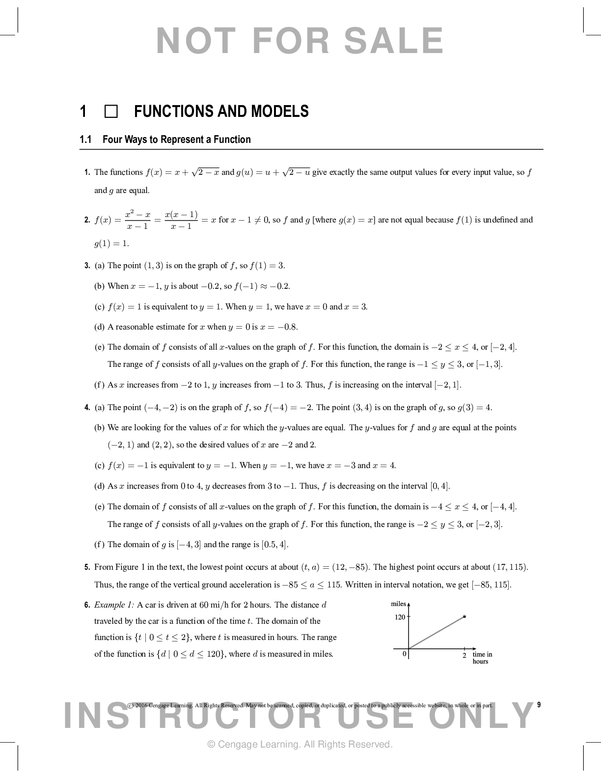
Buy this document to get the full access instantly
Instant Download Access after purchase
Add to cartInstant download
Reviews( 0 )
Document information
Connected school, study & course
About the document
Uploaded On
Jan 06, 2020
Number of pages
1
Written in

Additional information
This document has been written for:
Uploaded
Jan 06, 2020
Downloads
0
Views
82