Calculus > QUESTIONS & ANSWERS > Chapter 10: PARAMETRIC EQUATIONS AND POLAR COORDINATES. Work and Answers (All)
Chapter 10: PARAMETRIC EQUATIONS AND POLAR COORDINATES. Work and Answers
Document Content and Description Below
10.1 Curves Defined by Parametric Equations 1. = 1 − 2, = 2 − 2, −1 ≤ ≤ 2 −1 0 1 2 0 1 0 −3 −3 0 1 0 2. = 3 + , = 2 + 2, −2 ≤... ≤ 2 −2 −1 0 1 2 −10 −2 0 2 10 6 3 2 3 6 3. = + sin, = cos , − ≤ ≤ − −2 0 2 − −2 + 1 0 2 + 1 −1 0 1 0 −1 4. = − + , = − , −2 ≤ ≤ 2 −2 −1 0 1 2 2 − 2 539 − 1 172 1 −1 + 1 137 −2 + 2 214 −2 + 2 214 −1 + 1 137 1 − 1 172 2 − 2 539 5. = 2 − 1, = 1 2 + 1 (a) −4 −2 0 2 4 −9 −5 −1 3 7 −1 0 1 2 3 (b) = 2 − 1 ⇒ 2 = + 1 ⇒ = 1 2 + 1 2 , so = 1 2 + 1 = 1 2 1 2 + 1 2 + 1 = 1 4 + 1 4 + 1 ⇒ = 1 4 + 5 4 °c 2016 Cengage Learning. All Rights Reserved. May not be scanned, copied, or duplicated, or posted to a publicly accessible website, in whole or in part. 863 FOR INSTRUCTOR USE ONLY864 ¤ CHAPTER 10 PARAMETRIC EQUATIONS AND POLAR COORDINATES NOT FOR SALE 6. = 3 + 2, = 2 + 3 (a) −4 −2 0 2 4 −10 −4 2 8 14 −5 −1 3 7 11 (b) = 3 + 2 ⇒ 3 = − 2 ⇒ = 1 3 − 2 3 , so = 2 + 3 = 2 1 3 − 2 3 + 3 = 2 3 − 4 3 + 3 ⇒ = 2 3 + 5 3 7. = 2 − 3, = + 2, −3 ≤ ≤ 3 (a) −3 −1 1 3 6 −2 −2 6 −1 1 3 5 (b) = + 2 ⇒ = − 2, so = 2 − 3 = ( − 2)2 − 3 = 2 − 4 + 4 − 3 ⇒ = 2 − 4 + 1, −1 ≤ ≤ 5 8. = sin, = 1 − cos, 0 ≤ ≤ 2 (a) 0 2 32 2 0 1 0 −1 0 0 1 2 1 0 (b) = sin, = 1 − cos [or − 1 = −cos] ⇒ 2 + ( − 1)2 = (sin)2 + (−cos)2 ⇒ 2 + ( − 1)2 = 1. As varies from 0 to 2, the circle with center (01) and radius 1 is traced out. 9. = √, = 1 − (a) 0 1 2 3 4 0 1 1414 1732 2 1 0 −1 −2 −3 (b) = √ ⇒ = 2 ⇒ = 1 − = 1 − 2. Since ≥ 0, ≥ 0. So the curve is the right half of the parabola = 1 − 2. °c 2016 Cengage Learning. All Rights Reserved. May not be scanned, copied, or duplicated, or posted to a publicly accessible website, in whole or in part. FOR INSTRUCTOR USE ONLYNOT FORSECTION 10.1SALECURVES DEFINED BY PARAMETRIC EQUATIONS ¤ 865 10. = 2, = 3 (a) −2 −1 0 1 2 4 1 0 1 4 −8 −1 0 1 8 (b) = 3 ⇒ = 3 ⇒ = 2 = 3 2 = 23. ∈ R, ∈ R, ≥ 0. 11. (a) = sin 1 2, = cos 1 2, − ≤ ≤ . 2 + 2 = sin2 1 2 + cos2 1 2 = 1. For − ≤ ≤ 0, we have −1 ≤ ≤ 0 and 0 ≤ ≤ 1. For 0 ≤ , we have 0 ≤ 1 and 1 ≥ 0. The graph is a semicircle. (b) 12. (a) = 1 2 cos , = 2 sin, 0 ≤ ≤ . (2)2 + 1 22 = cos2 + sin2 = 1 ⇒ 42 + 1 42 = 1 ⇒ 2 (12)2 + 2 22 = 1, which is an equation of an ellipse with -intercepts ± 1 2 and -intercepts ±2. For 0 ≤ ≤ 2, we have 1 2 ≥ ≥ 0 and 0 ≤ ≤ 2. For 2 ≤ , we have 0 ≥ − 1 2 and 2 ≥ 0. So the graph is the top half of the ellipse. (b) 13. (a) = sin = csc, 0 2 . = csc = 1 sin = 1 . For 0 2 , we have 0 1 and 1. Thus, the curve is the portion of the hyperbola = 1 with 1. (b) 14. (a) = −2 = ()−2 = −2 = 12 for 0 since = . (b) °c 2016 Cengage Learning. All Rights Reserved. May not be scanned, copied, or duplicated, or posted to a publicly accessible website, in whole or in part. FOR INSTRUCTOR USE ONLY866 ¤ CHAPTER 10 PARAMETRIC EQUATIONS AND POLAR COORDINATES NOT FOR SALE 15. (a) = ln ⇒ = , so = 2 = ()2 = 2. (b) 16. (a) = √ + 1 ⇒ 2 = + 1 ⇒ = 2 − 1. = √ − 1 = (2 − 1) − 1 = √2 − 2. The curve is the part of the hyperbola 2 − 2 = 2 with ≥ √2 and ≥ 0. (b) 17. (a) = sinh, = cosh ⇒ 2 − 2 = cosh2 − sinh2 = 1. Since = cosh ≥ 1, we have the upper branch of the hyperbola 2 − 2 = 1. (b) 18. (a) = tan2 , = sec, −2 2. 1 + tan2 = sec2 ⇒ 1 + = 2 ⇒ = 2 − 1. For −2 ≤ 0, we have ≥ 0 and ≥ 1. For 0 2, we have 0 and 1 . Thus, the curve is the portion of the parabola = 2 − 1 in the first quadrant. As increases from −2 to 0, the point ( ) approaches (0 1) along the parabola. As increases from 0 to 2, the point ( ) retreats from (01) along the parabola. (b) 19. = 5 + 2 cos, = 3 + 2 sin ⇒ cos = − 5 2 , sin = −2 3. cos2() + sin2() = 1 ⇒ −2 52 + −2 32 = 1. The motion of the particle takes place on a circle centered at (5 3) with a radius 2. As goes from 1 to 2, the particle starts at the point (3 3) and moves counterclockwise along the circle −2 52 + −2 32 = 1 to (73) [one-half of a circle]. 20. = 2 + sin, = 1 + 3 cos ⇒ sin = − 2, cos = − 1 3 . sin2 + cos2 = 1 ⇒ ( − 2)2 + −3 12 = 1. The motion of the particle takes place on an ellipse centered at (2 1). As goes from 2 to 2, the particle starts at the point (31) and moves counterclockwise three-fourths of the way around the ellipse to (24). °c 2016 Cengage Learning. All Rights Reserved. May not be scanned, copied, or duplicated, or posted to a publicly accessible website, in whole or in part. FOR INSTRUCTOR USE ONLYNOT FORSECTION 10.1SALECURVES DEFINED BY PARAMETRIC EQUATIONS ¤ 867 21. = 5sin, = 2 cos ⇒ sin = 5, cos = 2 . sin2 + cos2 = 1 ⇒ 52 + 22 = 1. The motion of the particle takes place on an ellipse centered at (0 0). As goes from − to 5, the particle starts at the point (0 −2) and moves clockwise around the ellipse 3 times. 22. = cos2 = 1 − sin2 = 1 − 2. The motion of the particle takes place on the parabola = 1 − 2. As goes from −2 to −, the particle starts at the point (01), moves to (10), and goes back to (0 1). As goes from − to 0, the particle moves to (−10) and goes back to (01). The particle repeats this motion as goes from 0 to 2. 23. We must have 1 ≤ ≤ 4 and 2 ≤ ≤ 3. So the graph of the curve must be contained in the rectangle [1 4] by [23]. 24. (a) From the first graph, we have 1 ≤ ≤ 2. From the second graph, we have −1 ≤ ≤ 1 The only choice that satisfies either of those conditions is III. (b) From the first graph, the values of cycle through the values from −2 to 2 four times. From the second graph, the values of cycle through the values from −2 to 2 six times. Choice I satisfies these conditions. (c) From the first graph, the values of cycle through the values from −2 to 2 three times. From the second graph, we have 0 ≤ ≤ 2. Choice IV satisfies these conditions. (d) From the first graph, the values of cycle through the values from −2 to 2 two times. From the second graph, the values of do the same thing. Choice II satisfies these conditions. 25. When = −1, ( ) = (11). As increases to 0, and both decrease to 0. As increases from 0 to 1, increases from 0 to 1 and decreases from 0 to −1. As increases beyond 1, continues to increase and continues to decrease. For −1, and are both positive and decreasing. We could achieve greater accuracy by estimating - and -values for selected values of from the given graphs and plotting the corresponding points. 26. When = −1, ( ) = (00). As increases to 0, increases from 0 to 1, while first decreases to −1 and then increases to 0. As increases from 0 to 1, decreases from 1 to 0, while first increases to 1 and then decreases to 0. We could achieve greater accuracy by estimating - and -values for selected values of from the given graphs and plotting the corresponding points. y 0 1 x _1 1 t=_1, 1 (0, 0) t=0 (1, 0) 27. When = −1, ( ) = (01). As increases to 0, increases from 0 to 1 and decreases from 1 to 0. As increases from 0 to 1, the curve is retraced in the opposite direction with decreasing from 1 to 0 and increasing from 0 to 1. We could achieve greater accuracy by estimating - and -values for selected values of from the given graphs and plotting the corresponding points. °c 2016 Cengage Learning. All Rights Reserved. May not be scanned, copied, or duplicated, or posted to a publicly accessible website, in whole or in part. FOR INSTRUCTOR USE ONLY868 ¤ CHAPTER 10 PARAMETRIC EQUATIONS AND POLAR COORDINATES NOT FOR SALE 28. (a) = 4 − + 1 = (4 + 1) − 0 [think of the graphs of = 4 + 1 and = ] and = 2 ≥ 0, so these equations are matched with graph V. (b) = √ ≥ 0. = 2 − 2 = ( − 2) is negative for 0 2, so these equations are matched with graph I. (c) = sin 2 has period 22 = . Note that ( + 2) = sin[ + 2 + sin 2( + 2)] = sin( + 2 + sin 2) = sin( + sin 2) = (), so has period 2. These equations match graph II since cycles through the values −1 to 1 twice as cycles through those values once. (d) = cos 5 has period 25 and = sin 2 has period , so will take on the values −1 to 1, and then 1 to −1, before takes on the values −1 to 1. Note that when = 0, ( ) = (1 0). These equations are matched with graph VI (e) = + sin 4, = 2 + cos 3. As becomes large, and 2 become the dominant terms in the expressions for and , so the graph will look like the graph of = 2, but with oscillations. These equations are matched with graph IV. (f ) = sin 2 4 + 2 , = cos 2 4 + 2 . As → ∞, and both approach 0. These equations are matched with graph III. 29. Use = and = − 2sin with a -interval of [− ]. 30. Use 1 = , 1 = 3 − 4 and 2 = 3 − 4, 2 = with a -interval of [−33]. There are 9 points of intersection; (00) is fairly obvious. The point in quadrant I is approximately (2222), and by symmetry, the point in quadrant III is approximately (−22 −22). The other six points are approximately (∓19 ±05), (∓17 ±17), and (∓05 ±19). 31. (a) = 1 + (2 − 1), = 1 + (2 − 1), 0 ≤ ≤ 1. Clearly the curve passes through 1(1 1) when = 0 and through 2(2 2) when = 1. For 0 1, is strictly between 1 and 2 and is strictly between 1 and 2. For every value of , and satisfy the relation − 1 = 2 − 1 2 − 1 ( − 1), which is the equation of the line through 1(1 1) and 2(2 2). Finally, any point ( ) on that line satisfies − 1 2 − 1 = − 1 2 − 1 ; if we call that common value , then the given parametric equations yield the point ( ); and any ( ) on the line between 1(1 1) and 2(2 2) yields a value of in [01]. So the given parametric equations exactly specify the line segment from 1(1 1) to 2(2 2). (b) = −2 + [3 − (−2)] = −2 + 5 and = 7 + (−1 − 7) = 7 − 8 for 0 ≤ ≤ 1. °c 2016 Cengage Learning. All Rights Reserved. May not be scanned, copied, or duplicated, or posted to a publicly accessible website, in whole or in part. FOR INSTRUCTOR USE ONLYNOT FORSECTION 10.1SALECURVES DEFINED BY PARAMETRIC EQUATIONS ¤ 869 32. For the side of the triangle from to , use (1 1) = (11) and (2 2) = (42). Hence, the equations are = 1 + (2 − 1) = 1 + (4 − 1) = 1 + 3, = 1 + (2 − 1) = 1 + (2 − 1) = 1 + . Graphing = 1 + 3 and = 1 + with 0 ≤ ≤ 1 gives us the side of the triangle from to . Similarly, for the side we use = 4 − 3 and = 2 + 3, and for the side we use = 1 and = 1 + 4. 33. The circle 2 + ( − 1)2 = 4 has center (01) and radius 2, so by Example 4 it can be represented by = 2 cos, = 1 + 2 sin, 0 ≤ ≤ 2. This representation gives us the circle with a counterclockwise orientation starting at (21). (a) To get a clockwise orientation, we could change the equations to = 2 cos, = 1 − 2sin, 0 ≤ ≤ 2. (b) To get three times around in the counterclockwise direction, we use the original equations = 2 cos, = 1 + 2 sin with the domain expanded to 0 ≤ ≤ 6. (c) To start at (03) using the original equations, we must have 1 = 0; that is, 2cos = 0. Hence, = 2 . So we use = 2 cos, = 1 + 2 sin, 2 ≤ ≤ 32 . Alternatively, if we want to start at 0, we could change the equations of the curve. For example, we could use = −2sin, = 1 + 2 cos, 0 ≤ ≤ . 34. (a) Let 22 = sin2 and 22 = cos2 to obtain = sin and = cos with 0 ≤ ≤ 2 as possible parametric equations for the ellipse 22 + 22 = 1. (b) The equations are = 3 sin and = cos for ∈ {1 2 4 8}. (c) As increases, the ellipse stretches vertically. 35. Big circle: It’s centered at (2 2) with a radius of 2, so by Example 4, parametric equations are = 2 + 2cos = 2 + 2sin 0 ≤ ≤ 2 Small circles: They are centered at (13) and (33) with a radius of 01. By Example 4, parametric equations are (left) = 1 + 01cos = 3 + 01sin 0 ≤ ≤ 2 and (right) = 3 + 01cos = 3 + 01sin 0 ≤ ≤ 2 Semicircle: It’s the lower half of a circle centered at (2 2) with radius 1. By Example 4, parametric equations are = 2 + 1cos = 2 + 1sin ≤ ≤ 2 To get all four graphs on the same screen with a typical graphing calculator, we need to change the last -interval to[02] in order to match the others. We can do this by changing to 05. This change gives us the upper half. There are several ways to get the lower half—one is to change the “+” to a “−” in the -assignment, giving us = 2 + 1cos(05) = 2 − 1sin(05) 0 ≤ ≤ 2 °c 2016 Cengage Learning. All Rights Reserved. May not be scanned, copied, or duplicated, or posted to a publicly accessible website, in whole or in part. FOR INSTRUCTOR USE ONLY870 ¤ CHAPTER 10 PARAMETRIC EQUATIONS AND POLAR COORDINATES NOT FOR SALE 36. If you are using a calculator or computer that can overlay graphs (using multiple -intervals), the following is appropriate. Left side: = 1 and goes from 15 to 4, so use = 1 = 15 ≤ ≤ 4 Right side: = 10 and goes from 15 to 4, so use = 10 = 15 ≤ ≤ 4 Bottom: goes from 1 to 10 and = 15, so use = = 15 1 ≤ ≤ 10 Handle: It starts at (104) and ends at (13 7), so use = 10 + = 4 + 0 ≤ ≤ 3 Left wheel: It’s centered at (3 1), has a radius of 1, and appears to go about 30◦ above the horizontal, so use = 3 + 1 cos = 1 + 1 sin 56 ≤ ≤ 136 Right wheel: Similar to the left wheel with center (81), so use = 8 + 1 cos = 1 + 1 sin 56 ≤ ≤ 136 If you are using a calculator or computer that cannot overlay graphs (using one -interval), the following is appropriate. We’ll start by picking the -interval [025] since it easily matches the -values for the two sides. We now need to find parametric equations for all graphs with 0 ≤ ≤ 25. Left side: = 1 and goes from 15 to 4, so use = 1 = 15 + 0 ≤ ≤ 25 Right side: = 10 and goes from 15 to 4, so use = 10 = 15 + 0 ≤ ≤ 25 Bottom: goes from 1 to 10 and = 15, so use = 1 + 36 = 15 0 ≤ ≤ 25 To get the x-assignment, think of creating a linear function such that when = 0, = 1 and when = 25, = 10. We can use the point-slope form of a line with (1 1) = (01) and (2 2) = (25 10). − 1 = 10 − 1 25 − 0 ( − 0) ⇒ = 1 + 36. Handle: It starts at (104) and ends at (13 7), so use = 10 + 12 = 4 + 12 0 ≤ ≤ 25 (1 1) = (0 10) and (2 2) = (2513) gives us − 10 = 13 − 10 25 − 0 ( − 0) ⇒ = 10 + 12. (1 1) = (04) and (2 2) = (25 7) gives us − 4 = 7 − 4 25 − 0 ( − 0) ⇒ = 4 + 12. °c 2016 Cengage Learning. All Rights Reserved. May not be scanned, copied, or duplicated, or posted to a publicly accessible website, in whole or in part. FOR INSTRUCTOR USE ONLYNOT FORSECTION 10.1SALECURVES DEFINED BY PARAMETRIC EQUATIONS ¤ 871 Left wheel: It’s centered at (3 1), has a radius of 1, and appears to go about 30◦ above the horizontal, so use = 3 + 1 cos 815 + 56 = 1 + 1 sin 815 + 56 0 ≤ ≤ 25 (1 1) = 0 56 and (2 2) = 5 2 136 gives us − 56 = 13 6 − 5 6 5 2 − 0 ( − 0) ⇒ = 56 + 815 . Right wheel: Similar to the left wheel with center (81), so use = 8 + 1 cos 815 + 56 = 1 + 1 sin 815 + 56 0 ≤ ≤ 25 37. (a) = 3 ⇒ = 13, so = 2 = 23. We get the entire curve = 23 traversed in a left to right direction. (b) = 6 ⇒ = 16, so = 4 = 46 = 23. Since = 6 ≥ 0, we only get the right half of the curve = 23. (c) = −3 = (−)3 [so − = 13], = −2 = (−)2 = (13)2 = 23. If 0, then and are both larger than 1. If 0, then and are between 0 and 1. Since 0 and 0, the curve never quite reaches the origin. 38. (a) = , so = −2 = −2. We get the entire curve = 12 traversed in a left-to-right direction. (b) = cos, = sec2 = 1 cos2 = 1 2 . Since sec ≥ 1, we only get the parts of the curve = 12 with ≥ 1. We get the first quadrant portion of the curve when 0, that is, cos 0, and we get the second quadrant portion of the curve when 0, that is, cos 0. (c) = , = −2 = ()−2 = −2. Since and −2 are both positive, we only get the first quadrant portion of the curve = 12. °c 2016 Cengage Learning. All Rights Reserved. May not be scanned, copied, or duplicated, or posted to a publicly accessible website, in whole or in part. FOR INSTRUCTOR USE ONLY872 ¤ CHAPTER 10 PARAMETRIC EQUATIONS AND POLAR COORDINATES NOT FOR SALE 39. The case 2 is illustrated. has coordinates ( ) as in Example 7, and has coordinates ( + cos( − )) = ( (1 − cos)) [since cos( − ) = cos cos + sin sin = −cos], so has coordinates ( − sin( − ) (1 − cos)) = (( − sin) (1 − cos )) [since sin( − ) = sin cos − cos sin = sin]. Again we have the parametric equations = ( − sin), = (1 − cos). 40. The first two diagrams depict the case 32 , . As in Example 7, has coordinates ( ). Now (in the second diagram) has coordinates ( + cos( − )) = ( − cos), so a typical point of the trochoid has coordinates ( + sin( − ) − cos ). That is, has coordinates ( ), where = − sin and = − cos. When = , these equations agree with those of the cycloid. 41. It is apparent that = || and = || = ||. From the diagram, = || = cos and = || = sin. Thus, the parametric equations are = cos and = sin. To eliminate we rearrange: sin = ⇒ sin2 = ()2 and cos = ⇒ cos2 = ()2. Adding the two equations: sin2 + cos2 = 1 = 22 + 22. Thus, we have an ellipse. 42. has coordinates (cos sin). Since is perpendicular to , ∆ is a right triangle and has coordinates (sec0). It follows that has coordinates (sec sin ). Thus, the parametric equations are = sec, = sin. 43. = (2cot2), so the -coordinate of is = 2cot . Let = (02). Then ∠ is a right angle and ∠ = , so || = 2sin and = ((2sin)cos (2sin)sin). Thus, the -coordinate of is = 2sin2 . 44. (a) Let be the angle of inclination of segment . Then || = 2 cos. Let = (20). Then by use of right triangle we see that || = 2cos. Now || = || = || − || = 2cos 1 − cos = 2 1 −cos cos 2 = 2 sin cos2 = 2sin tan So has coordinates = 2sin tan · cos = 2sin2 and = 2sin tan · sin = 2sin2 tan. (b) °c 2016 Cengage Learning. All Rights Reserved. May not be scanned, copied, or duplicated, or posted to a publicly accessible website, in whole or in part. FOR INSTRUCTOR USE ONLYNOT FORSECTION 10.1SALECURVES DEFINED BY PARAMETRIC EQUATIONS ¤ 873 45. (a) There are 2 points of intersection: (−3 0) and approximately (−2114). (b) A collision point occurs when 1 = 2 and 1 = 2 for the same . So solve the equations: 3sin = −3 + cos (1) 2cos = 1 + sin (2) From (2), sin = 2 cos − 1. Substituting into (1), we get 3(2 cos − 1) = −3 + cos ⇒ 5cos = 0 () ⇒ cos = 0 ⇒ = 2 or 32 . We check that = 32 satisfies (1) and (2) but = 2 does not. So the only collision point occurs when = 3 2 , and this gives the point (−30). [We could check our work by graphing 1 and 2 together as functions of and, on another plot, 1 and 2 as functions of . If we do so, we see that the only value of for which both pairs of graphs intersect is = 32 .] (c) The circle is centered at (31) instead of (−31). There are still 2 intersection points: (30) and (2114), but there are no collision points, since () in part (b) becomes 5cos = 6 ⇒ cos = 6 5 1. 46. (a) If = 30◦ and 0 = 500 ms, then the equations become = (500 cos 30◦) = 250√3 and = (500 sin 30◦) − 1 2(98)2 = 250 − 492. = 0 when = 0 (when the gun is fired) and again when = 250 49 ≈ 51 s. Then = 250√3 250 49 ≈ 22,092 m, so the bullet hits the ground about 22 km from the gun. The formula for is quadratic in . To find the maximum -value, we will complete the square: = −492 − 250 49 = −492 − 250 49 + 125 49 2 + 125 492 = −49 − 125 49 2 + 125 492 ≤ 125 492 with equality when = 125 49 s, so the maximum height attained is 125 492 ≈ 3189 m. (b) As (0◦ 90◦) increases up to 45◦, the projectile attains a greater height and a greater range. As increases past 45◦, the projectile attains a greater height, but its range decreases. (c) = (0 cos) ⇒ = 0 cos . = (0 sin) − 1 22 ⇒ = (0 sin) 0 cos − 2 0 cos 2 = (tan) − 202 cos 2 2, which is the equation of a parabola (quadratic in ). °c 2016 Cengage Learning. All Rights Reserved. May not be scanned, copied, or duplicated, or posted to a publicly accessible website, in whole or in part. FOR INSTRUCTOR USE ONLY874 ¤ CHAPTER 10 PARAMETRIC EQUATIONS AND POLAR COORDINATES NOT FOR SALE 47. = 2 = 3 − . We use a graphing device to produce the graphs for various values of with − ≤ ≤ . Note that all the members of the family are symmetric about the -axis. For 0, the graph does not cross itself, but for = 0 it has a cusp at (00) and for 0 the graph crosses itself at = , so the loop grows larger as increases. 48. = 2 − 43 = −2 + 34. We use a graphing device to produce the graphs for various values of with − ≤ ≤ . Note that all the members of the family are symmetric about the -axis. When 0, the graph resembles that of a polynomial of even degree, but when = 0 there is a corner at the origin, and when 0, the graph crosses itself at the origin, and has two cusps below the -axis. The size of the “swallowtail” increases as increases. 49. = + cos = + sin 0. From the first figure, we see that curves roughly follow the line = , and they start having loops when is between 14 and 16. The loops increase in size as increases. While not required, the following is a solution to determine the exact values for which the curve has a loop, that is, we seek the values of for which there exist parameter values and such that and ( + cos + sin) = ( + cos + sin). In the diagram at the left, denotes the point ( ), the point ( ), and the point ( + cos + sin) = ( + cos + sin). Since = = , the triangle is isosceles. Therefore its base angles, = ∠ and = ∠ are equal. Since = − 4 and = 2 − 34 − = 54 − , the relation = implies that + = 3 2 (1). °c 2016 Cengage Learning. All Rights Reserved. May not be scanned, copied, or duplicated, or posted to a publicly accessible website, in whole or in part. FOR INSTRUCTOR USE ONLYNOT FORSECTION 10.1SALECURVES DEFINED BY PARAMETRIC EQUATIONS ¤ 875 Since = distance(( )( )) = 2( − )2 = √2( − ), we see that cos = 1 2 = ( − )√2 , so − = √2cos, that is, − = √2cos − 4 (2). Now cos − 4 = sin 2 − − 4 = sin 34 − , so we can rewrite (2) as − = √2sin 34 − (20). Subtracting (20) from (1) and dividing by 2, we obtain = 34 − √22sin 34 − , or 34 − = √2 sin 34 − (3). Since 0 and , it follows from (20) that sin 34 − 0. Thus from (3) we see that 34 . [We have implicitly assumed that 0 by the way we drew our diagram, but we lost no generality by doing so since replacing by + 2 merely increases and by 2. The curve’s basic shape repeats every time we change by 2.] Solving for in (3), we get = √2 34 − sin 34 − . Write = 34 − . Then = √2 sin , where 0. Now sin for 0, so √2. As → 0+, that is, as → 34 − , → √2. 50. Consider the curves = sin + sin, = cos + cos, where is a positive integer. For = 1, we get a circle of radius 2 centered at the origin. For 1, we get a curve lying on or inside that circle that traces out − 1 loops as ranges from 0 to 2. Note: 2 + 2 = (sin + sin)2 + (cos + cos)2 = sin2 + 2sin sin + sin2 + cos2 + 2cos cos + cos2 = (sin2 + cos2 ) + (sin2 + cos2 ) + 2(cos cos + sin sin) = 1 + 1 + 2cos( − ) = 2 + 2cos((1 − )) ≤ 4 = 22, with equality for = 1. This shows that each curve lies on or inside the curve for = 1, which is a circle of radius 2 centered at the origin. = 1 = 2 = 3 = 5 51. Note that all the Lissajous figures are symmetric about the -axis. The parameters and simply stretch the graph in the - and -directions respectively. For = = = 1 the graph is simply a circle with radius 1. For = 2 the graph crosses °c 2016 Cengage Learning. All Rights Reserved. May not be scanned, copied, or duplicated, or posted to a publicly accessible website, in whole or in part. FOR INSTRUCTOR USE ONLY876 ¤ CHAPTER 10 PARAMETRIC EQUATIONS AND POLAR COORDINATES NOT FOR SALE itself at the origin and there are loops above and below the -axis. In general, the figures have − 1 points of intersection, all of which are on the -axis, and a total of closed loops. = = 1 = 2 = 3 52. = cos, = sin − sin. If = 1, then = 0, and the curve is simply the line segment from (−10) to (10). The graphs are shown for = 234 and 5. It is easy to see that all the curves lie in the rectangle [−11] by [−22]. When is an integer, ( + 2) = () and ( + 2) = (), so the curve is closed. When is a positive integer greater than 1, the curve intersects the x-axis + 1 times and has loops (one of which degenerates to a tangency at the origin when is an odd integer of the form 4 + 1). As increases, the curve’s loops become thinner, but stay in the region bounded by the semicircles = ±1 + √1 − 2 and the line segments from (−1 −1) to (−11) and from (1 −1) to (11). This is true because || = |sin − sin| ≤ |sin| + |sin| ≤ √1 − 2 + 1. This curve appears to fill the entire region when is very large, as shown in the figure for = 1000. °c 2016 Cengage Learning. All Rights Reserved. May not be scanned, copied, or duplicated, or posted to a publicly accessible website, in whole or in part. FOR INSTRUCTOR USE ONLYNOT FORLABORATORY PROJECT SALERUNNING CIRCLES AROUND CIRCLES ¤ 877 When is a fraction, we get a variety of shapes with multiple loops, but always within the same region. For some fractional values, such as = 2359, the curve again appears to fill the region. LABORATORY PROJECT Running Circles Around Circles 1. The center of the smaller circle has coordinates (( − )cos ( − )sin). Arc on circle has length since it is equal in length to arc (the smaller circle rolls without slipping against the larger.) Thus, ∠ = and ∠ = − , so has coordinates = ( − )cos + cos(∠ ) = ( − )cos + cos − and = ( − )sin − sin(∠ ) = ( − )sin − sin − . 2. With = 1 and a positive integer greater than 2, we obtain a hypocycloid of cusps. Shown in the figure is the graph for = 4. Let = 4 and = 1. Using the sum identities to expand cos 3 and sin 3, we obtain = 3 cos + cos 3 = 3 cos + 4cos3 − 3cos = 4cos3 and = 3sin − sin3 = 3sin − 3sin − 4sin3 = 4sin3 . 3. The graphs at the right are obtained with = 1 and = 1 2, 1 3 , 1 4 , and 10 1 with −2 ≤ ≤ 2. We conclude that as the denominator increases, the graph gets smaller, but maintains the basic shape shown. [continued] °c 2016 Cengage Learning. All Rights Reserved. May not be scanned, copied, or duplicated, or posted to a publicly accessible website, in whole or in part. FOR INSTRUCTOR USE ONLY878 ¤ CHAPTER 10 PARAMETRIC EQUATIONS AND POLAR COORDINATES NOT FOR SALE Letting = 2 and = 3, 5, and 7 with −2 ≤ ≤ 2 gives us the following: So if is held constant and varies, we get a graph with cusps (assuming is in lowest form). When = + 1, we obtain a hypocycloid of cusps. As increases, we must expand the range of in order to get a closed curve. The following graphs have = 3 2, 5 4, and 11 10. 4. If = 1, the equations for the hypocycloid are = ( − 1)cos + cos(( − 1)) = ( − 1)sin − sin(( − 1)) which is a hypocycloid of cusps (from Problem 2). In general, if 1, we get a figure with cusps on the “outside ring” and if 1, the cusps are on the “inside ring”. In any case, as the values of get larger, we get a figure that looks more and more like a washer. If we were to graph the hypocycloid for all values of , every point on the washer would eventually be arbitrarily close to a point on the curve. = √2, −10 ≤ ≤ 10 = − 2, 0 ≤ ≤ 446 5. The center of the smaller circle has coordinates (( + )cos( + )sin). Arc has length (as in Problem 1), so that ∠ = , ∠ = − , and ∠ = − − = − + since ∠ = . Thus, the coordinates of are = ( + )cos + cos − + = ( + )cos − cos + and = ( + )sin − sin − + = ( + )sin − sin + . °c 2016 Cengage Learning. All Rights Reserved. May not be scanned, copied, or duplicated, or posted to a publicly accessible website, in whole or in part. FOR INSTRUCTOR USE ONLYNOT FORLABORATORY PROJECT SALERUNNING CIRCLES AROUND CIRCLES ¤ 879 6. Let = 1 and the equations become = ( + 1)cos − cos(( + 1)) = ( + 1) sin − sin(( + 1)) If = 1, we have a cardioid. If is a positive integer greater than 1, we get the graph of an “-leafed clover”, with cusps that are units from the origin. (Some of the pairs of figures are not to scale.) = 3, −2 ≤ ≤ 2 = 10, −2 ≤ ≤ 2 If = with = 1, we obtain a figure that does not increase in size and requires − ≤ ≤ to be a closed curve traced exactly once. = 1 4, −4 ≤ ≤ 4 = 1 7, −7 ≤ ≤ 7 Next, we keep constant and let vary. As increases, so does the size of the figure. There is an -pointed star in the middle. = 2 5, −5 ≤ ≤ 5 = 7 5, −5 ≤ ≤ 5 Now if = + 1 we obtain figures similar to the previous ones, but the size of the figure does not increase. = 4 3, −3 ≤ ≤ 3 = 7 6, −6 ≤ ≤ 6 If is irrational, we get washers that increase in size as increases. = √2, 0 ≤ ≤ 200 = − 2, 0 ≤ ≤ 446 °c 2016 Cengage Learning. All Rights Reserved. May not be scanned, copied, or duplicated, or posted to a publicly accessible website, in whole or in part. FOR INSTRUCTOR USE ONLY880 ¤ CHAPTER 10 PARAMETRIC EQUATIONS AND POLAR COORDINATES NOT FOR SALE 10.2 Calculus with Parametric Curves 1. = 1 + , = √1 + ⇒ = 1 2(1 + )−12 = 2√1 + 1 , = (1 +(1 + )(1))−2 (1) = (1 +1 )2 , and = = 1(2√1 + ) 1(1 + )2 = (1 + )2 2√1 + = 1 2 (1 + )32. 2. = , = + sin ⇒ = 1 + cos, = + = ( + 1), and = = 1 + cos ( + 1) . 3. = 3 + 1, = 4 + ; = −1. = 43 + 1, = 32, and = = 43 3+ 1 2 . When = −1, ( ) = (00) and = −33 = −1, so an equation of the tangent to the curve at the point corresponding to = −1 is − 0 = −1( − 0), or = −. 4. = √, = 2 − 2; = 4. = 2 − 2, = 2√1 , and = = (2 − 2)2√ = 4( − 1)√. When = 4, ( ) = (28) and = 4(3)(2) = 24, so an equation of the tangent to the curve at the point corresponding to = 4 is − 8 = 24( − 2), or = 24 − 40. 5. = cos, = sin; = . = cos + sin, = (−sin) + cos, and = = −cos sin+ sin + cos. When = , ( ) = (−0) and = −(−1) = , so an equation of the tangent to the curve at the point corresponding to = is − 0 = [ − (−)], or = + 2. 6. = sin, = 2; = 0. = 22, = ( cos) + (sin) = ( cos + sin), and = = 22 ( cos + sin) = 2 cos + sin. When = 0, ( ) = (01) and = 2, so an equation of the tangent to the curve at the point corresponding to = 0 is − 1 = 2 ( − 0), or = 2 + 1. 7. (a) = 1 + ln, = 2 + 2; (1 3). = 2 = 1 and = = 12 = 22. At (13), = 1 + ln = 1 ⇒ ln = 0 ⇒ = 1 and = 2, so an equation of the tangent is − 3 = 2( − 1), or = 2 + 1. (b) = 1 + ln ⇒ ln = − 1 ⇒ = −1, so = 2 + 2 = (−1)2 + 2 = 2−2 + 2, and 0 = 2−2 · 2. At (13), 0 = 2(1)−2 · 2 = 2, so an equation of the tangent is − 3 = 2( − 1), or = 2 + 1. 8. (a) = 1 + √, = 2; (2 ). = 2 · 2, = 2√1 , and = = 12 2√2 = 4322. At (2 ), = 1 + √ = 2 ⇒ √ = 1 ⇒ = 1 and = 4, so an equation of the tangent is − = 4( − 2), or = 4 − 7. °c 2016 Cengage Learning. All Rights Reserved. May not be scanned, copied, or duplicated, or posted to a publicly accessible website, in whole or in part. FOR INSTRUCTOR USE ONLYNOT FORSECTION 10.2 SALECALCULUS WITH PARAMETRIC CURVES ¤ 881 (b) = 1 + √ ⇒ √ = − 1 ⇒ = ( − 1)2, so = 2 = (−1)4, and 0 = (−1)4 · 4( − 1)3. At (2 ), 0 = · 4 = 4, so an equation of the tangent is − = 4( − 2), or = 4 − 7. 9. = 2 − , = 2 + + 1; (03). = = 2 + 1 2 − 1 . To find the value of corresponding to the point (03), solve = 0 ⇒ 2 − = 0 ⇒ ( − 1) = 0 ⇒ = 0 or = 1. Only = 1 gives = 3. With = 1, = 3, and an equation of the tangent is − 3 = 3( − 0), or = 3 + 3. 10. = sin, = 2 + ; (0 2). = = 2 + 1 cos . To find the value of corresponding to the point (02), solve = 2 ⇒ 2 + − 2 = 0 ⇒ ( + 2)( − 1) = 0 ⇒ = −2 or = 1. Either value gives = −3, so an equation of the tangent is − 2 = − 3 ( − 0), or = − 3 + 2. 11. = 2 + 1, = 2 + ⇒ = = 2 + 1 2 = 1 + 1 2 ⇒ 2 2 = = −1(22) 2 = − 1 43 . The curve is CU when 2 2 0, that is, when 0. 12. = 3 + 1, = 2 − ⇒ = = 2 − 1 32 = 2 3 − 1 32 ⇒ 2 2 = = − 2 32 + 2 33 32 = 2 − 2 33 32 = 2(1 − ) 95 . The curve is CU when 22 0, that is, when 0 1. 13. = , = − ⇒ = = −− + − = −(1 − ) = −2(1 − ) ⇒ 2 2 = = −2(−1) + (1 − )(−2−2) = −2(−1 − 2 + 2) = −3(2 − 3). The curve is CU when 2 2 0, that is, when 3 2. 14. = 2 + 1, = − 1 ⇒ = = 2 ⇒ 2 2 = = 2 − · 2 (2)2 2 = 2( − 1) (2)3 = ( − 1) 43 . The curve is CU when 2 2 0, that is, when 0 or 1. °c 2016 Cengage Learning. All Rights Reserved. May not be scanned, copied, or duplicated, or posted to a publicly accessible website, in whole or in part. FOR INSTRUCTOR USE ONLY882 ¤ CHAPTER 10 PARAMETRIC EQUATIONS AND POLAR COORDINATES NOT FOR SALE 15. = − ln, = + ln [note that 0] ⇒ = = 1 + 1 1 − 1 = + 1 − 1 ⇒ 2 2 = = ( − 1)(1) − ( + 1)(1) ( − 1)2 ( − 1) = −2 ( − 1)3 . The curve is CU when 22 0, that is, when 0 1. 16. = cos, = sin 2, 0 ⇒ = = 2cos 2 −sin ⇒ 2 2 = = (−sin)(−4sin 2) − (2 cos 2)(−cos) (−sin)2 −sin = (sin)(8 sin cos) + [2(1 − 2sin2 )](cos) (−sin)sin2 = (cos )(8 sin2 + 2 − 4sin2 ) (−sin)sin2 = − cos sin · 4sin2 + 2 sin2 [ (−cot) · positive expression] The curve is CU when 2 2 0, that is, when −cot 0 ⇔ cot 0 ⇔ 2 . 17. = 3 − 3, = 2 − 3. = 2, so = 0 ⇔ = 0 ⇔ ( ) = (0 −3). = 32 − 3 = 3( + 1)( − 1), so = 0 ⇔ = −1 or 1 ⇔ ( ) = (2 −2) or (−2 −2). The curve has a horizontal tangent at (0 −3) and vertical tangents at (2 −2) and (−2 −2). 18. = 3 − 3, = 3 − 32. = 32 − 6 = 3( − 2), so = 0 ⇔ = 0 or 2 ⇔ ( ) = (00) or (2 −4). = 32 − 3 = 3( + 1)( − 1), so = 0 ⇔ = −1 or 1 ⇔ ( ) = (2 −4) or (−2 −2). The curve has horizontal tangents at (00) and (2 −4), and vertical tangents at (2 −4) and (−2 −2). 19. = cos, = cos 3. The whole curve is traced out for 0 ≤ ≤ . = −3sin 3, so = 0 ⇔ sin 3 = 0 ⇔ 3 = 0, , 2, or 3 ⇔ = 0, 3 , 23 , or ⇔ ( ) = (11), 1 2 −1, − 1 21, or (−1 −1). = −sin, so = 0 ⇔ sin = 0 ⇔ = 0 or ⇔ ( ) = (11) or (−1 −1). Both and equal 0 when = 0 and . To find the slope when = 0, we find lim →0 = lim →0 −−3sin 3 sin = lim H →0 −−9cos 3 cos = 9, which is the same slope when = . Thus, the curve has horizontal tangents at 1 2 −1 and − 1 2 1, and there are no vertical tangents. °c 2016 Cengage Learning. All Rights Reserved. May not be scanned, copied, or duplicated, or posted to a publicly accessible website, in whole or in part. FOR INSTRUCTOR USE ONLYNOT FORSECTION 10.2 SALECALCULUS WITH PARAMETRIC CURVES ¤ 883 20. = sin , = cos . The whole curve is traced out for 0 ≤ 2. = −sin cos , so = ⇔ sin = 0 ⇔ = 0 or ⇔ ( ) = (1 ) or (1 1). = cos sin , so = 0 ⇔ cos = 0 ⇔ = 2 or 32 ⇔ ( ) = (1) or (11). The curve has horizontal tangents at (1 ) and (1 1), and vertical tangents at (1) and (1 1). 21. From the graph, it appears that the rightmost point on the curve = − 6, = is about (06 2). To find the exact coordinates, we find the value of for which the graph has a vertical tangent, that is, 0 = = 1 − 65 ⇔ = 1√5 6. Hence, the rightmost point is 1√5 6 − 1 6 √5 6 1 √5 6 = 5 · 6−65 6−15 ≈ (058201). 22. From the graph, it appears that the lowest point and the leftmost point on the curve = 4 − 2, = + 4 are (15 −05) and (−1212), respectively. To find the exact coordinates, we solve = 0 (horizontal tangents) and = 0 (vertical tangents). = 0 ⇔ 1 + 43 = 0 ⇔ = − √314, so the lowest point is √3 256 1 + √324 − √314 + √3 256 1 = √3 256 9 − √3 256 3 ≈ (142 −047). = 0 ⇔ 43 − 2 = 0 ⇔ = √312, so the leftmost point is √3116 − √322 √312 + √3116 = − √3316 √3316 ≈ (−119119). 23. We graph the curve = 4 − 23 − 22, = 3 − in the viewing rectangle [−211] by [−0505]. This rectangle corresponds approximately to ∈ [−108]. We estimate that the curve has horizontal tangents at about (−1 −04) and (−017 039) and vertical tangents at about (00) and (−019037). We calculate = = 32 − 1 43 − 62 − 4. The horizontal tangents occur when = 32 − 1 = 0 ⇔ = ± √13 , so both horizontal tangents are shown in our graph. The vertical tangents occur when °c 2016 Cengage Learning. All Rights Reserved. May not be scanned, copied, or duplicated, or posted to a publicly accessible website, in whole or in part. FOR INSTRUCTOR USE ONLY884 ¤ CHAPTER 10 PARAMETRIC EQUATIONS AND POLAR COORDINATES NOT FOR SALE = 2(22 − 3 − 2) = 0 ⇔ 2(2 + 1)( − 2) = 0 ⇔ = 0, − 1 2 or 2. It seems that we have missed one vertical tangent, and indeed if we plot the curve on the -interval [−12 22] we see that there is another vertical tangent at (−86). 24. We graph the curve = 4 + 43 − 82, = 22 − in the viewing rectangle [−3702] by [−0214]. It appears that there is a horizontal tangent at about (−04 −01), and vertical tangents at about (−3 1) and (0 0). We calculate = = 4 − 1 43 + 122 − 16, so there is a horizontal tangent where = 4 − 1 = 0 ⇔ = 1 4 . This point (the lowest point) is shown in the first graph. There are vertical tangents where = 43 + 122 − 16 = 0 ⇔ 4(2 + 3 − 4) = 0 ⇔ 4( + 4)( − 1) = 0. We have missed one vertical tangent corresponding to = −4, and if we plot the graph for ∈ [−5 3], we see that the curve has another vertical tangent line at approximately (−12836). 25. = cos, = sincos. = −sin, = −sin2 + cos2 = cos 2. ( ) = (00) ⇔ cos = 0 ⇔ is an odd multiple of 2 . When = 2 , = −1 and = −1, so = 1. When = 3 2 , = 1 and = −1. So = −1. Thus, = and = − are both tangent to the curve at (0 0). 26. = −2cos, = sin + sin 2. From the graph, it appears that the curve crosses itself at the point (10). If this is true, then = 1 ⇔ −2cos = 1 ⇔ cos = − 1 2 ⇔ = 23 or 43 for 0 ≤ ≤ 2. Substituting either value of into gives = 0, confirming that (10) is the point where the curve crosses itself. = = cos + 2 cos 2 2sin . When = 2 3 , = −12 + 2(−12) 2(√32) = −32 √3 = − √3 2 , so an equation of the tangent line is − 0 = − √3 2 ( − 1), or = − √3 2 + √3 2 . Similarly, when = 4 3 , an equation of the tangent line is = √3 2 − √3 2 . 27. = − sin, = − cos. (a) = − cos, = sin, so = −sin cos . (b) If 0 , then |cos| ≤ , so − cos ≥ − 0. This shows that never vanishes, so the trochoid can have no vertical tangent if . °c 2016 Cengage Learning. All Rights Reserved. May not be scanned, copied, or duplicated, or posted to a publicly accessible website, in whole or in part. FOR INSTRUCTOR USE ONLYNOT FORSECTION 10.2 SALECALCULUS WITH PARAMETRIC CURVES ¤ 885 28. = cos3 , = sin3 . (a) = −3cos2 sin, = 3sin2 cos, so = −cos sin = −tan. (b) The tangent is horizontal ⇔ = 0 ⇔ tan = 0 ⇔ = ⇔ ( ) = (±0). The tangent is vertical ⇔ cos = 0 ⇔ is an odd multiple of 2 ⇔ ( ) = (0 ±) (c) = ±1 ⇔ tan = ±1 ⇔ is an odd multiple of 4 ⇔ ( ) = ± √42 ± √42 [All sign choices are valid.] 29. = 32 + 1, = 3 − 1 ⇒ = = 32 6 = 2 . The tangent line has slope 1 2 when 2 = 1 2 ⇔ = 1, so the point is (40). 30. = 32 + 1, = 23 + 1, = 6, = 62, so = 662 = [even where = 0]. So at the point corresponding to parameter value , an equation of the tangent line is − (23 + 1) = [ − (32 + 1)]. If this line is to pass through (4 3), we must have 3 − (23 + 1) = [4 − (32 + 1)] ⇔ 23 − 2 = 33 − 3 ⇔ 3 − 3 + 2 = 0 ⇔ ( − 1)2( + 2) = 0 ⇔ = 1 or −2. Hence, the desired equations are − 3 = − 4, or = − 1, tangent to the curve at (43), and − (−15) = −2( − 13), or = −2 + 11, tangent to the curve at (13 −15). 31. By symmetry of the ellipse about the - and -axes, = 40 = 4 0 2 sin (−sin) = 4 02 sin2 = 4 02 12(1 − cos 2) = 2 − 1 2 sin 2 0 2 = 2 2 = 32. The curve = 2 − 2 = ( − 2), = √ intersects the -axis when = 0, that is, when = 0 and = 2. The corresponding values of are 0 and √2. The shaded area is given by =0 =√2( − ) = =0 =2 [0 − ()]0() = − 02(2 − 2)2√1 = − 02 1 232 − 12 = − 1 552 − 2 3322 0 = − 1 5 · 252 − 2 3 · 232 = −212 4 5 − 4 3 = −√2− 15 8 = 15 8 √2 33. The curve = 3 + 1, = 2 − 2 = (2 − ) intersects the -axis when = 0, that is, when = 0 and = 2. The corresponding values of are 1 and 9. The shaded area is given by =1 =9( − ) = =0 =2[() − 0] 0() = 02(2 − 2)(32) = 302(23 − 4) = 3 1 24 − 1 552 0 = 38 − 32 5 = 24 5 °c 2016 Cengage Learning. All Rights Reserved. May not be scanned, copied, or duplicated, or posted to a publicly accessible website, in whole or in part. FOR INSTRUCTOR USE ONLY886 ¤ CHAPTER 10 PARAMETRIC EQUATIONS AND POLAR COORDINATES NOT FOR SALE 34. By symmetry, = 40 = 4 0 2 sin3 (−3cos2 sin) = 122 02 sin4 cos2 . Now sin4 cos2 = sin2 1 4 sin2 2 = 1 8 (1 − cos 2)sin2 2 = 1 8 1 2(1 − cos 4) − sin2 2 cos 2 = 16 1 − 64 1 sin 4 − 48 1 sin3 2 + so 02 sin4 cos2 = 16 1 − 64 1 sin 4 − 48 1 sin3 2 0 2 = 32 . Thus, = 122 32 = 3 82. 35. = − sin, = − cos. = 02 = 02( − cos)( − cos ) = 02(2 − 2 cos + 2 cos2 ) = 2 − 2 sin + 1 22 + 1 2 sin 22 0 = 22 + 2 36. (a) By symmetry, the area of R is twice the area inside R above the -axis. The top half of the loop is described by = 2, = 3 − 3, −√3 ≤ ≤ 0, so, using the Substitution Rule with = 3 − 3 and = 2 , we find that area = 203 = 20−√3(3 − 3)2 = 20−√3(24 − 62) = 2 2 55 − 23− 0 √3 = 2 2 5(−312)5 − 2(−312)3 = 2 2 5 −9√3 − 2−3√3 = 24 5 √3 (b) Here we use the formula for disks and use the Substitution Rule as in part (a): volume = 03 2 = 0−√3(3 − 3)22 = 2 0−√3(6 − 64 + 92) = 2 1 88 − 6 + 9 44− 0 √3 = 2 1 8(−312)8 − (−312)6 + 9 4(−312)4 = 2 81 8 − 27 + 81 4 = 27 4 (c) By symmetry, the -coordinate of the centroid is 0. To find the -coordinate, we note that it is the same as the -coordinate of the centroid of the top half of R, the area of which is 1 2 · 24 5 √3 = 12 5 √3. So, using Formula 8.3.8 with = 12 5 √3, we get = 5 12√3 03 = 125√3 0−√3 2(3 − 3)2 = 6√5 3 1 77 − 3 55− 0 √3 = 5 6√3 1 7(−312)7 − 3 5(−312)5 = 6√5 3 − 27 7 √3 + 27 5 √3 = 9 7 So the coordinates of the centroid of R are ( ) = 9 70. 37. = + −, = − −, 0 ≤ ≤ 2. = 1 − − and = 1 + −, so ()2 + ()2 = (1 − −)2 + (1 + −)2 = 1 − 2− + −2 + 1 + 2− + −2 = 2 + 2−2. Thus, = ()2 + ()2 = 02 √2 + 2−2 ≈ 31416. 38. = 2 − , = 4, 1 ≤ ≤ 4 = 2 − 1 and = 43, so ()2 + ()2 = (2 − 1)2 + (43)2 = 42 − 4 + 1 + 166. Thus, = ()2 + ()2 = 14 √166 + 42 − 4 + 1 ≈ 2553756. 39. = − 2sin, = 1 − 2cos, 0 ≤ ≤ 4. = 1 − 2cos and = 2 sin, so ()2 + ()2 = (1 − 2cos )2 + (2 sin)2 = 1 − 4cos + 4 cos2 + 4 sin2 = 5 − 4cos . Thus, = ()2 + ()2 = 04 √5 − 4cos ≈ 267298. °c 2016 Cengage Learning. All Rights Reserved. May not be scanned, copied, or duplicated, or posted to a publicly accessible website, in whole or in part. FOR INSTRUCTOR USE ONLYNOT FORSECTION 10.2 SALECALCULUS WITH PARAMETRIC CURVES ¤ 887 40. = + √, = − √, 0 ≤ ≤ 1. = 1 + 2√1 and = 1 − 2√1 , so 2 + 2 = 1 + 2√1 2 + 1 − 2√1 2 = 1 + √1 + 41 + 1 − √1 + 41 = 2 + 21. Thus, = ()2 + ()2 = 01 2 + 21 = lim →0+ 1 2 + 21 ≈ 20915. 41. = 1 + 32, = 4 + 23, 0 ≤ ≤ 1. = 6 and = 62, so ()2 + ()2 = 362 + 364. Thus, = 01 362 + 364 = 01 6 1 + 2 = 612 √ 1 2 [ = 1 + 2, = 2 ] = 3 2 3322 1 = 2(232 − 1) = 22√2 − 1 42. = − , = 42, 0 ≤ ≤ 2. = − 1 and = 22, so ()2 + ()2 = ( − 1)2 + (22)2 = 2 − 2 + 1 + 4 = 2 + 2 + 1 = ( + 1)2. Thus, = 02 ( + 1)2 = 02 + 1 = 02( + 1) = + 2 0 = (2 + 2) − (1 + 0) = 2 + 1. 43. = sin, = cos, 0 ≤ ≤ 1. = cos + sin and = −sin + cos, so 2 + 2 = 2 cos2 + 2 sin cos + sin2 + 2 sin2 − 2sin cos + cos2 = 2(cos2 + sin2 ) + sin2 + cos2 = 2 + 1. Thus, = 01 √2 + 1 =21 1 2√2 + 1 + 1 2 ln + √2 + 11 0 = 1 2√2 + 1 2 ln1 + √2. 44. = 3 cos − cos 3, = 3 sin − sin 3, 0 ≤ ≤ . = −3sin + 3 sin 3 and = 3 cos − 3cos 3, so 2 + 2 = 9 sin2 − 18 sin sin 3 + 9 sin2(3) + 9 cos2 − 18 cos cos 3 + 9 cos2(3) = 9(cos2 + sin2 ) − 18(cos cos 3 + sin sin 3) + 9[cos2(3) + sin2(3)] = 9(1) − 18 cos( − 3) + 9(1) = 18 − 18 cos(−2) = 18(1 − cos 2) = 18[1 − (1 − 2sin2 )] = 36 sin2 . Thus, = 0 √36 sin2 = 60 |sin| = 60 sin = −6cos 0 = −6(−1 − 1) = 12. 45. = cos , = sin, 0 ≤ ≤ . 2 + 2 = [(cos − sin)]2 + [(sin + cos)]2 = ()2(cos2 − 2cos sin + sin2 ) + ()2(sin2 + 2 sin cos + cos2 = 2(2 cos2 + 2 sin2 ) = 22 Thus, = 0 √22 = 0 √2 = √2 0 = √2( − 1). °c 2016 Cengage Learning. All Rights Reserved. May not be scanned, copied, or duplicated, or posted to a publicly accessible website, in whole or in part. FOR INSTRUCTOR USE ONLY888 ¤ CHAPTER 10 PARAMETRIC EQUATIONS AND POLAR COORDINATES NOT FOR SALE 46. = cos + ln(tan 1 2), = sin, 4 ≤ ≤ 34. = −sin + 1 2 sec2(2) tan(2) = −sin + 2sin(2) cos( 1 2) = −sin + sin 1 and = cos , so 2 + 2 = sin2 − 2 + sin12 + cos2 = 1 − 2 + csc2 = cot2 . Thus, = 3 4 4 |cot| = 2 42 cot = 2ln|sin| 2 4 = 2ln 1 − ln √12 = 20 + ln√2 = 2 1 2 ln 2 = ln 2. 47. The figure shows the curve = sin + sin 15, = cos for 0 ≤ ≤ 4. = cos + 15cos 15 and = −sin, so ()2 + ()2 = cos2 + 3 cos cos 15 + 225 cos2 15 + sin2 . Thus, = 04 √1 + 3 cos cos 15 + 225 cos2 15 ≈ 167102. 48. = 3 − 3, = 32. = 3 − 32 and = 6, so 2 + 2 = (3 − 32)2 + (6)2 = (3 + 32)2 and the length of the loop is given by = −√√33 (3 + 32) = 20√3 (3 + 32) = 23 + 3√ 0 3 = 23√3 + 3√3 = 12√3 49. = − , = + , −6 ≤ ≤ 6. 2 + 2 = (1 − )2 + (1 + )2 = (1 − 2 + 2) + (1 + 2 + 2) = 2 + 22, so = −66 √2 + 22 . Set () = √2 + 22. Then by Simpson’s Rule with = 6 and ∆ = 6−(6−6) = 2, we get ≈ 2 3[(−6) + 4(−4) + 2(−2) + 4(0) + 2(2) + 4(4) + (6)] ≈ 6123053. 50. = 2cot ⇒ = −2csc2 and = 2sin2 ⇒ = 4sin cos = 2sin 2. So = 42 42 csc4 + 42 sin2 2 = 2 42 csc4 + sin2 2 . Using Simpson’s Rule with = 4, ∆ = 2−4 4 = 16 , and () = csc4 + sin2 2, we get ≈ 2 · 4 = (2) 16·3 4 + 4 516 + 2 38 + 4 716 + 2 ≈ 22605. 51. = sin2 , = cos2 , 0 ≤ ≤ 3. ()2 + ()2 = (2 sin cos)2 + (−2cossin)2 = 8 sin2 cos2 = 2 sin2 2 ⇒ °c 2016 Cengage Learning. All Rights Reserved. May not be scanned, copied, or duplicated, or posted to a publicly accessible website, in whole or in part. FOR INSTRUCTOR USE ONLYNOT FORSECTION 10.2 SALECALCULUS WITH PARAMETRIC CURVES ¤ 889 Distance = 03 √2|sin 2| = 6√202 sin 2 [by symmetry] = −3√2cos 2 0 2 = −3√2(−1 − 1) = 6√2. The full curve is traversed as goes from 0 to 2 , because the curve is the segment of + = 1 that lies in the first quadrant (since , ≥ 0), and this segment is completely traversed as goes from 0 to 2 . Thus, = 02 sin 2 = √2, as above. 52. = cos2 , = cos , 0 ≤ ≤ 4. 2 + 2 = (−2cos sin)2 + (−sin)2 = sin2 (4 cos2 + 1) Distance = 04 |sin| √4cos2 + 1 = 40 sin √4cos2 + 1 = −41−1 √42 + 1 [ = cos, = −sin ] = 4−11 √42 + 1 = 801 √42 + 1 = 80tan−1 2 sec · 1 2 sec2 [2 = tan 2 = sec2 ] = 40tan−1 2 sec3 =71 2sec tan + 2 ln|sec + tan|tan 0 −1 2 = 4√5 + 2 ln√5 + 2 Thus, = 0 |sin| √4cos2 + 1 = √5 + 1 2 ln√5 + 2. 53. = sin, = cos, 0 ≤ ≤ 2. 2 + 2 = (cos)2 + (−sin)2 = 2 cos2 + 2 sin2 = 2(1 − sin2 ) + 2 sin2 = 2 − (2 − 2) sin2 = 2 − 2 sin2 = 21 − 22 sin2 = 2(1 − 2 sin2 ) So = 402 2 1 − 2 sin2 [by symmetry] = 4 02 1 − 2 sin2 . 54. = cos3 , = sin3 . 2 + 2 = (−3cos2 sin)2 + (3sin2 cos)2 = 92 cos4 sin2 + 92 sin4 cos2 = 92 sin2 cos2 (cos2 + sin2 ) = 92 sin2 cos2 . The graph has four-fold symmetry and the curve in the first quadrant corresponds to 0 ≤ ≤ 2. Thus, = 402 3sin cos [since 0 and sin and cos are positive for 0 ≤ ≤ 2] = 12 1 2 sin2 0 2 = 12 1 2 − 0 = 6 55. (a) = 11 cos − 4cos(112), = 11 sin − 4sin(112). Notice that 0 ≤ ≤ 2 does not give the complete curve because (0) 6= (2). In fact, we must take ∈ [04] in order to obtain the complete curve, since the first term in each of the parametric equations has period 2 and the second has period 11 22 = 411 , and the least common integer multiple of these two numbers is 4. °c 2016 Cengage Learning. All Rights Reserved. May not be scanned, copied, or duplicated, or posted to a publicly accessible website, in whole or in part. FOR INSTRUCTOR USE ONLY890 ¤ CHAPTER 10 PARAMETRIC EQUATIONS AND POLAR COORDINATES NOT FOR SALE (b) We use the CAS to find the derivatives and , and then use Theorem 5 to find the arc length. Recent versions of Maple express the integral 04 ()2 + ()2 as 882√2, where () is the elliptic integral 01 √√11−−222 and is the imaginary number √−1. Some earlier versions of Maple (as well as Mathematica) cannot do the integral exactly, so we use the command evalf(Int(sqrt(diff(x,t)ˆ2+diff(y,t)ˆ2),t=0..4*Pi)); to estimate the length, and find that the arc length is approximately 29403. Derive’s Para_arc_length function in the utility file Int_apps simplifies the integral to 1104 −4cos cos 11 2 − 4sin sin 11 2 + 5. 56. (a) It appears that as → ∞, ( ) → 1 2 1 2 , and as → −∞, ( ) → − 1 2 − 1 2 . (b) By the Fundamental Theorem of Calculus, = cos 2 2 and = sin 2 2, so by Theorem 5, the length of the curve from the origin to the point with parameter value is = 0 2 + 2 = 0 cos2 2 2 + sin2 2 2 = 0 1 = [or − if 0] We have used as the dummy variable so as not to confuse it with the upper limit of integration. 57. = sin, = cos, 0 ≤ ≤ 2. = cos + sin and = −sin + cos, so ()2 + ()2 = 2 cos2 + 2sin cos + sin2 + 2 sin2 − 2sin cos + cos2 = 2(cos2 + sin2 ) + sin2 + cos2 = 2 + 1 = 2 = 02 2cos√2 + 1 ≈ 47394. 58. = sin, = sin2, 0 ≤ ≤ 2. = cos and = 2cos2, so ()2 + ()2 = cos2 + 4cos2 2. = 2 = 02 2 sin2√cos2 + 4cos2 2 ≈ 80285. 59. = + , = −, 0 ≤ ≤ 1. = 1 + and = −−, so ()2 + ()2 = (1 + )2 + (−−)2 = 1 + 2 + 2 + −2. = 2 = 01 2−√1 + 2 + 2 + −2 ≈ 106705. 60. = 2 − 3, = + 4, 0 ≤ ≤ 1. ()2 + ()2 = (2 − 32)2 + (1 + 43)2 = 42 − 123 + 94 + 1 + 83 + 166, so = 2 = 01 2( + 4)√166 + 94 − 43 + 42 + 1 ≈ 127176. °c 2016 Cengage Learning. All Rights Reserved. May not be scanned, copied, or duplicated, or posted to a publicly accessible website, in whole or in part. FOR INSTRUCTOR USE ONLYNOT FORSECTION 10.2 SALECALCULUS WITH PARAMETRIC CURVES ¤ 891 61. = 3, = 2, 0 ≤ ≤ 1. 2 + 2 = 322 + (2)2 = 94 + 42. = 01 2 2 + 2 = 01 2294 + 42 = 2 01 22(92 + 4) = 2 413 −9 4 √ 18 1 = 9 = 18 2 + 4, so , 2 = ( = 18 −1 4) 9, = 92·18 413(32 − 412) = 81 2 552 − 8 33213 4 = 81 · 15 2 352 − 203213 4 = 2 1215 3 · 132 √13 − 20 · 13√13 − (3 · 32 − 20 · 8) = 1215 2 247√13 + 64 62. = 22 + 1, = 8√, 1 ≤ ≤ 3. 2 + 2 = 4 − 12 2 + √42 = 162 − 8 + 14 + 16 = 162 + 8 + 14 = 4 + 12 2. = 13 2 2 + 2 = 13 28√ 4 + 12 2 = 16 13 12(4 + −2) = 16 13(432 + −32) = 16 8 552 − 2−123 1 = 16 72 5 √3 − 2 3√3 − ( 8 5 − 2) = 16 206 15 √3 + 15 6 = 32 15103√3 + 3 63. = cos3 , = sin3 , 0 ≤ ≤ 2 . 2 + 2 = (−3cos2 sin)2 + (3sin2 cos)2 = 92 sin2 cos2 . = 02 2 · sin3 · 3sin cos = 62 02 sin4 cos = 6 52sin5 0 2 = 6 52 64. = 2 cos − cos 2, = 2 sin − sin 2 ⇒ 2 + 2 = (−2sin + 2 sin 2)2 + (2 cos − 2cos 2)2 = 4[(sin2 − 2sin sin 2 + sin2 2) + (cos2 − 2cos cos 2 + cos2 2)] = 4[1 + 1 − 2(cos 2 cos + sin 2 sin)] = 8[1 − cos(2 − )] = 8(1 − cos) We plot the graph with parameter interval [02], and see that we should only integrate between 0 and . (If the interval [02] were taken, the surface of revolution would be generated twice.) Also note that = 2 sin − sin 2 = 2 sin(1 − cos ). So = 0 2 · 2sin(1 − cos)2√2√1 − cos = 8√2 0 (1 − cos)32 sin = 8√2 02 √3 = 1 = sin− cos = 8√2 2 5 522 0 = 16 5 √2(252) = 128 5 65. = 32, = 23, 0 ≤ ≤ 5 ⇒ 2 + 2 = (6)2 + (62)2 = 362(1 + 2) ⇒ = 05 2 ()2 + ()2 = 05 2(32)6 √1 + 2 = 18 05 2√1 + 2 2 = 18 126 ( − 1)√ = 1 + = 2 2 = 18 126(32 − 12) = 18 2 552 − 2 33226 1 = 18 2 5 · 676√26 − 2 3 · 26√26 − 2 5 − 2 3 = 24 5 949√26 + 1 °c 2016 Cengage Learning. All Rights Reserved. May not be scanned, copied, or duplicated, or posted to a publicly accessible website, in whole or in part. FOR INSTRUCTOR USE ONLY892 ¤ CHAPTER 10 PARAMETRIC EQUATIONS AND POLAR COORDINATES NOT FOR SALE 66. = − , = 42, 0 ≤ ≤ 1. 2 + 2 = ( − 1)2 + (22)2 = 2 + 2 + 1 = ( + 1)2. = 01 2( − )( − 1)2 + (22)2 = 01 2( − )( + 1) = 2 1 22 + − ( − 1) − 1 221 0 = (2 + 2 − 6) 67. If 0 is continuous and 0() 6= 0 for ≤ ≤ , then either 0() 0 for all in [ ] or 0() 0 for all in [ ]. Thus, is monotonic (in fact, strictly increasing or strictly decreasing) on [ ]. It follows that has an inverse. Set = ◦ −1, that is, define by () = (−1()). Then = () ⇒ −1() = , so = () = (−1()) = (). 68. By Formula 8.2.5 with = (), = 2()1 + [ 0()]2 . But by Formula 10.2.1, 1 + [ 0()]2 = 1 + 2 = 1 + 2 = ( ( )2 + () 2 )2 . Using the Substitution Rule with = (), where = () and = (), we have since = = 2 (())( ( )2 + () 2 )2 = 2 2 + 2 , which is Formula 10.2.6. 69. (a) = tan−1 ⇒ = tan−1 = 1 + ( 1 )2 . But = = ˙˙ ⇒ = ˙˙ = ¨˙ −˙ 2 ¨˙ ⇒ = 1 + (1 ˙ ˙)2 ¨˙ −˙ 2 ¨˙ = ˙˙¨2 −+ ¨˙2˙ . Using the Chain Rule, and the fact that = 0 2 + 2 ⇒ = 2 + 2 = ˙ 2 + ˙212, we have that = = ˙˙¨2 −+ ¨˙2˙ (˙ 2 +1˙2)12 = (˙2˙¨+−˙2¨)˙32 . So = = (˙2˙¨+−˙2¨)˙32 = (˙|2˙¨+−˙2¨)˙3|2 . (b) = and = () ⇒ ˙ = 1, ¨ = 0 and ˙ = , ¨ = 22 . So = 1 · (22) − 0 · () [1 + ()2]32 = 22 [1 + ()2]32 . 70. (a) = 2 ⇒ = 2 ⇒ 22 = 2. So = [1 + ( 22)2 ]32 = (1 + 422)32 , and at (11), = 2 532 = 2 5√5. (b) 0 = = −3(1 + 42)−52(8) = 0 ⇔ = 0 ⇒ = 0. This is a maximum since 0 0 for 0 and 0 0 for 0. So the parabola = 2 has maximum curvature at the origin. 71. = − sin ⇒ ˙ = 1 − cos ⇒ ¨ = sin, and = 1 − cos ⇒ ˙ = sin ⇒ ¨ = cos. Therefore, = cos − cos2 − sin2 [(1 − cos)2 + sin2 ]32 = cos − (cos2 + sin2 ) (1 − 2cos + cos2 + sin2 )32 = |cos − 1| (2 − 2cos)32 . The top of the arch is °c 2016 Cengage Learning. All Rights Reserved. May not be scanned, copied, or duplicated, or posted to a publicly accessible website, in whole or in part. FOR INSTRUCTOR USE ONLYNOT FORSECTION 10.2 SALECALCULUS WITH PARAMETRIC CURVES ¤ 893 characterized by a horizontal tangent, and from Example 2(b) in Section 10.2, the tangent is horizontal when = (2 − 1), so take = 1 and substitute = into the expression for : = |cos − 1| (2 − 2cos)32 = |−1 − 1| [2 − 2(−1)]32 = 1 4 . 72. (a) Every straight line has parametrizations of the form = + , = + , where , are arbitrary and , 6= 0. For example, a straight line passing through distinct points ( ) and ( ) can be described as the parametrized curve = + ( − ), = + ( − ). Starting with = + , = + , we compute ˙ = , ˙ = , ¨ = ¨ = 0, and = | · 0 − · 0| (2 + 2)32 = 0. (b) Parametric equations for a circle of radius are = cos and = sin. We can take the center to be the origin. So ˙ = − sin ⇒ ¨ = − cos and ˙ = cos ⇒ ¨ = − sin. Therefore, = 2 sin2 + 2 cos2 (2 sin2 + 2 cos2 )32 = 2 3 = 1 . And so for any (and thus any point), = 1 . 73. The coordinates of are ( cos sin). Since was unwound from arc , has length . Also ∠ = ∠ − ∠ = 1 2 − , so has coordinates = cos + cos 1 2 − = (cos + sin), = sin − sin 1 2 − = (sin − cos). 74. If the cow walks with the rope taut, it traces out the portion of the involute in Exercise 73 corresponding to the range 0 ≤ ≤ , arriving at the point (− ) when = . With the rope now fully extended, the cow walks in a semicircle of radius , arriving at (− −). Finally, the cow traces out another portion of the involute, namely the reflection about the -axis of the initial involute path. (This corresponds to the range − ≤ ≤ 0.) Referring to the figure, we see that the total grazing area is 2(1 + 3). 3 is one-quarter of the area of a circle of radius , so 3 = 1 4 ()2 = 1 4 32. We will compute 1 + 2 and then subtract 2 = 1 2 2 to obtain 1. To find 1 + 2, first note that the rightmost point of the involute is 2 . [To see this, note that = 0 when = 0 or 2 . = 0 corresponds to the cusp at ( 0) and = 2 corresponds to 2 .] The leftmost point of the involute is (− ). Thus, 1 + 2 = =2 − =02 = 0= . Now = (sin − cos) cos = 2( sin cos − 2 cos2 ). Integrate: (12) = − cos2 − 1 22 − 1sin cos − 1 6 3 + 1 2 + . This enables us to compute °c 2016 Cengage Learning. All Rights Reserved. May not be scanned, copied, or duplicated, or posted to a publicly accessible website, in whole or in part. FOR INSTRUCTOR USE ONLY894 ¤ CHAPTER 10 PARAMETRIC EQUATIONS AND POLAR COORDINATES NOT FOR SALE 1 + 2 = 2− cos2 − 1 2(2 − 1) sin cos − 1 63 + 1 20 = 20 − − − 63 + 2 = 22 + 63 Therefore, 1 = (1 + 2) − 2 = 1 632, so the grazing area is 2(1 + 3) = 2 1 632 + 1 432 = 5 632. LABORATORY PROJECT Bézier Curves 1. The parametric equations for a cubic Bézier curve are = 0(1 − )3 + 31(1 − )2 + 322(1 − ) + 33 = 0(1 − )3 + 31(1 − )2 + 322(1 − ) + 33 where 0 ≤ ≤ 1. We are given the points 0(0 0) = (4 1), 1(1 1) = (2848), 2(2 2) = (50 42), and 3(3 3) = (405). The curve is then given by () = 4(1 − )3 + 3 · 28(1 − )2 + 3 · 502(1 − ) + 403 () = 1(1 − )3 + 3 · 48(1 − )2 + 3 · 422(1 − ) + 53 where 0 ≤ ≤ 1. The line segments are of the form = 0 + (1 − 0), = 0 + (1 − 0): 01 = 4 + 24, = 1 + 47 12 = 28 + 22, = 48 − 6 23 = 50 − 10, = 42 − 37 2. It suffices to show that the slope of the tangent at 0 is the same as that of line segment 01, namely 1 − 0 1 − 0 . We calculate the slope of the tangent to the Bézier curve: = −30(1 − )2 + 31−2(1 − ) + (1 − )2 + 32−2 + (2)(1 − ) + 332 −32 0(1 − ) + 31[−2(1 − ) + (1 − )2] + 32[−2 + (2)(1 − )] + 332 At point 0, = 0, so the slope of the tangent is −30 + 31 −30 + 31 = 1 − 0 1 − 0 . So the tangent to the curve at 0 passes through 1. Similarly, the slope of the tangent at point 3 [where = 1] is −32 + 33 −32 + 33 = 3 − 2 3 − 2 , which is also the slope of line 23. 3. It seems that if 1 were to the right of 2, a loop would appear. We try setting 1 = (110 30), and the resulting curve does indeed have a loop. 4. Based on the behavior of the Bézier curve in Problems 1–3, we suspect that the four control points should be in an exaggerated C shape. We try 0(1012), 1(415), 2(45), and 3(108), and these produce a decent C. If you are using a CAS, it may be necessary to instruct it to make the - and -scales the same so as not to distort the figure (this is called a “constrained projection” in Maple.) °c 2016 Cengage Learning. All Rights Reserved. May not be scanned, copied, or duplicated, or posted to a publicly accessible website, in whole or in part. FOR INSTRUCTOR USE ONLYNOT FOR SALESECTION 10.3 POLAR COORDINATES ¤ 895 5. We use the same 0 and 1 as in Problem 4, and use part of our C as the top of an S. To prevent the center line from slanting up too much, we move 2 up to (46) and 3 down and to the left, to (87). In order to have a smooth joint between the top and bottom halves of the S (and a symmetric S), we determine points 4, 5, and 6 by rotating points 2, 1, and 0 about the center of the letter (point 3). The points are therefore 4(128), 5(12 −1), and 6(62). 10.3 Polar Coordinates 1. (a) 1 4 By adding 2 to 4 , we obtain the point 1 94 , which satisfies the 0 requirement. The direction opposite 4 is 54, so −1 54 is a point that satisfies the 0 requirement. (b) −2 32 0: −(−2) 32 − = 2 2 0: −2 32 + 2 = −2 72 (c) 3 − 3 0: 3 − 3 + 2 = 3 53 0: −3 − 3 + = −3 23 2. (a) 2 56 0: 2 56 + 2 = 2 176 0: −2 56 − = −2 − 6 (b) 1 − 23 0:1 − 23 + 2 = 1 43 0: −1 − 23 + = −1 3 (c) −1 54 0: −(−1) 54 − = 1 4 0: −1 54 − 2 = −1 − 34 °c 2016 Cengage Learning. All Rights Reserved. May not be scanned, copied, or duplicated, or posted to a publicly accessible website, in whole or in part. FOR INSTRUCTOR USE ONLY896 ¤ CHAPTER 10 PARAMETRIC EQUATIONS AND POLAR COORDINATES NOT FOR SALE 3. (a) = 2cos 32 = 2(0) = 0 and = 2 sin 32 = 2(−1) = −2 give us the Cartesian coordinates (0 −2). (b) = √2cos 4 = √2√12 = 1 and = √2sin 4 = √2√12 = 1 give us the Cartesian coordinates (11). (c) = −1cos−6 = −1√23 = −√23 and = −1sin−6 = −1−12 = 12 give us the Cartesian coordinates −√23 12. 4. (a) = 4 cos 4 3 = 4−21 = −2 and = 4 sin 4 3 = 4−√23 = −2√3 give us the Cartesian coordinates −2 −2√3. (b) = −2cos 3 4 = −2−√22 = √2 and = −2sin 3 4 = −2√22 = −√2 give us the Cartesian coordinates √2 −√2. (c) = −3cos−3 = −312 = −32 and = −3sin−3 = −3−√23 = 3√23 give us the Cartesian coordinates −3 2 3√23. 5. (a) = −4 and = 4 ⇒ = (−4)2 + 42 = 4√2 and tan = −44 = −1 [ = − 4 + ]. Since (−44) is in the second quadrant, the polar coordinates are (i) 4√2 34 and (ii) −4√2 74 . °c 2016 Cengage Learning. All Rights Reserved. May not be scanned, copied, or duplicated, or posted to a publicly accessible website, in whole or in part. FOR INSTRUCTOR USE ONLYNOT FOR SALESECTION 10.3 POLAR COORDINATES ¤ 897 (b) = 3 and = 3√3 ⇒ = 32 + 3√32 = √9 + 27 = 6 and tan = 3√33 = √3 [ = 3 + ]. Since 33√3 is in the first quadrant, the polar coordinates are (i) 6 3 and (ii) −6 43 . 6. (a) = √3 and = −1 ⇒ = √32 + (−1)2 = 2 and tan = √−13 [ = − 6 + ]. Since √3 −1 is in the fourth quadrant, the polar coordinates are (i) 2 116 and (ii) −2 56 . (b) = −6 and = 0 ⇒ = (−6)2 + 02 = 6 and tan = −06 = 0 [ = ]. Since (−60) is on the negative -axis, the polar coordinates are (i) (6 ) and (ii) (−60). 7. ≥ 1. The curve = 1 represents a circle with center and radius 1. So ≥ 1 represents the region on or outside the circle. Note that can take on any value. 8. 0 ≤ 2, ≤ ≤ 32. This is the region inside the circle = 2 in the third quadrant. 9. ≥ 0, 4 ≤ ≤ 34. = represents a line through . 10. 1 ≤ ≤ 3, 6 56 11. 2 3, 53 ≤ ≤ 73 12. ≥ 1, ≤ ≤ 2 13. Converting the polar coordinates 4 43 and 6 53 to Cartesian coordinates gives us 4cos 43 4sin 43 = −2 −2√3 and 6cos 53 6sin 53 = 3 −3√3. Now use the distance formula = (2 − 1)2 + (2 − 1)2 = [3 − (−2)]2 + −3√3 − −2√32 = 52 + −√32 = √25 + 3 = √28 = 2√7 °c 2016 Cengage Learning. All Rights Reserved. May not be scanned, copied, or duplicated, or posted to a publicly accessible website, in whole or in part. FOR INSTRUCTOR USE ONLY898 ¤ CHAPTER 10 PARAMETRIC EQUATIONS AND POLAR COORDINATES NOT FOR SALE 14. The points (1 1) and (2 2) in Cartesian coordinates are (1 cos1 1 sin1) and (2 cos2 2 sin2), respectively. The square of the distance between them is (2 cos2 − 1 cos1)2 + (2 sin2 − 1 sin1)2 = 22 cos2 2 − 212 cos1 cos2 + 12 cos2 1 + 22 sin2 2 − 212 sin1 sin2 + 12 sin2 1 = 12sin2 1 + cos2 1 + 22sin2 2 + cos2 2 − 212(cos1 cos2 + sin1 sin2) = 12 − 212 cos(1 − 2) + 22, so the distance between them is 12 − 212 cos(1 − 2) + 22. 15. 2 = 5 ⇔ 2 + 2 = 5, a circle of radius √5 centered at the origin. 16. = 4 sec ⇔ sec = 4 ⇔ cos = 4 ⇔ = 4, a vertical line. 17. = 5 cos ⇒ 2 = 5 cos ⇔ 2 + 2 = 5 ⇔ 2 − 5 + 25 4 + 2 = 25 4 ⇔ − 5 2 2 + 2 = 25 4 , a circle of radius 5 2 centered at 5 2 0. The first two equations are actually equivalent since 2 = 5 cos ⇒ ( − 5cos) = 0 ⇒ = 0 or = 5 cos. But = 5 cos gives the point = 0 (the pole) when = 0. Thus, the equation = 5 cos is equivalent to the compound condition ( = 0 or = 5 cos). 18. = 3 ⇒ tan = tan 3 ⇒ = √3 ⇔ = √3, a line through the origin. 19. 2 cos 2 = 1 ⇔ 2(cos2 − sin2 ) = 1 ⇔ ( cos)2 − ( sin)2 = 1 ⇔ 2 − 2 = 1, a hyperbola centered at the origin with foci on the -axis. 20. 2 sin 2 = 1 ⇔ 2(2 sin cos) = 1 ⇔ 2( cos)( sin) = 1 ⇔ 2 = 1 ⇔ = 1 2, a hyperbola centered at the origin with foci on the line = . 21. = 2 ⇔ sin = 2 ⇔ = 2 sin ⇔ = 2 csc 22. = ⇒ = 1 [ 6= 0] ⇒ tan = 1 ⇒ = tan−1 1 ⇒ = 4 or = 54 [either includes the pole] 23. = 1 + 3 ⇔ sin = 1 + 3 cos ⇔ sin − 3 cos = 1 ⇔ (sin − 3cos) = 1 ⇔ = 1 sin − 3cos 24. 42 = ⇔ 4( sin)2 = cos ⇔ 42 sin2 − cos = 0 ⇔ (4 sin2 − cos) = 0 ⇔ = 0 or = cos 4sin2 ⇔ = 0 or = 1 4 cot csc. = 0 is included in = 1 4 cot csc when = 2 , so the curve is represented by the single equation = 1 4 cot csc. 25. 2 + 2 = 2 ⇔ 2 = 2 cos ⇔ 2 − 2 cos = 0 ⇔ ( − 2cos) = 0 ⇔ = 0 or = 2cos. = 0 is included in = 2cos when = 2 + , so the curve is represented by the single equation = 2cos °c 2016 Cengage Learning. All Rights Reserved. May not be scanned, copied, or duplicated, or posted to a publicly accessible website, in whole or in part. FOR INSTRUCTOR USE ONLYNOT FOR SALESECTION 10.3 POLAR COORDINATES ¤ 899 26. 2 − 2 = 4 ⇔ ( cos )2 − ( sin)2 = 4 ⇔ 2 cos2 − 2 sin2 = 4 ⇔ 2(cos2 − sin2 ) = 4 ⇔ 2 cos 2 = 4 27. (a) The description leads immediately to the polar equation = 6 , and the Cartesian equation = tan 6 = √13 is slightly more difficult to derive. (b) The easier description here is the Cartesian equation = 3. 28. (a) Because its center is not at the origin, it is more easily described by its Cartesian equation, ( − 2)2 + ( − 3)2 = 52. (b) This circle is more easily given in polar coordinates: = 4. The Cartesian equation is also simple: 2 + 2 = 16. 29. = −2sin 30. = 1 − cos 31. = 2(1 + cos) 32. = 1 + 2 cos °c 2016 Cengage Learning. All Rights Reserved. May not be scanned, copied, or duplicated, or posted to a publicly accessible website, in whole or in part. FOR INSTRUCTOR USE ONLY900 ¤ CHAPTER 10 PARAMETRIC EQUATIONS AND POLAR COORDINATES NOT FOR SALE 33. = , ≥ 0 34. = 2, −2 ≤ ≤ 2 35. = 3cos3 36. = −sin5 37. = 2cos4 38. = 2sin6 °c 2016 Cengage Learning. All Rights Reserved. May not be scanned, copied, or duplicated, or posted to a publicly accessible website, in whole or in part. FOR INSTRUCTOR USE ONLYNOT FOR SALESECTION 10.3 POLAR COORDINATES ¤ 901 39. = 1 + 3cos 40. = 1 + 5sin 41. 2 = 9sin2 42. 2 = cos4 43. = 2 + sin3 °c 2016 Cengage Learning. All Rights Reserved. May not be scanned, copied, or duplicated, or posted to a publicly accessible website, in whole or in part. FOR INSTRUCTOR USE ONLY902 ¤ CHAPTER 10 PARAMETRIC EQUATIONS AND POLAR COORDINATES NOT FOR SALE 44. 2 = 1 ⇔ = ±1√ for 0 45. = sin(2) 46. = cos(3) 47. For = 0, , and 2, has its minimum value of about 05. For = 2 and 32 , attains its maximum value of 2. We see that the graph has a similar shape for 0 ≤ ≤ and ≤ ≤ 2. 48. The given graph has a maximum of 2 for = 0, a minimum of 1 for = 4 , and then a maximum of 2 for = 2 . This pattern is repeated 4 times for 0 ≤ ≤ 2. °c 2016 Cengage Learning. All Rights Reserved. May not be scanned, copied, or duplicated, or posted to a publicly accessible website, in whole or in part. FOR INSTRUCTOR USE ONLYNOT FOR SALESECTION 10.3 POLAR COORDINATES ¤ 903 49. = cos = (4 + 2sec)cos = 4cos + 2. Now, → ∞ ⇒ (4 + 2 sec) → ∞ ⇒ → 2 − or → 32 + [since we need only consider 0 ≤ 2], so lim →∞ = lim →2− (4 cos + 2) = 2. Also, → −∞ ⇒ (4 + 2 sec) → −∞ ⇒ → 2 + or → 32 −, so lim →−∞ = lim →2+ (4 cos + 2) = 2. Therefore, lim →±∞ = 2 ⇒ = 2 is a vertical asymptote. 50. = sin = 2 sin − csc sin = 2 sin − 1. → ∞ ⇒ (2 − csc) → ∞ ⇒ csc → −∞ ⇒ → + [since we need only consider 0 ≤ 2] and so lim →∞ = lim →+ 2sin − 1 = −1. Also → −∞ ⇒ (2 − csc) → −∞ ⇒ csc → ∞ ⇒ → − and so lim →−∞ = lim →− 2sin − 1 = −1. Therefore lim →±∞ = −1 ⇒ = −1 is a horizontal asymptote. 51. To show that = 1 is an asymptote we must prove lim →±∞ = 1. = ()cos = (sin tan)cos = sin2 . Now, → ∞ ⇒ sin tan → ∞ ⇒ → 2 −, so lim →∞ = lim →2− sin2 = 1. Also, → −∞ ⇒ sin tan → −∞ ⇒ → 2 +, so lim →−∞ = lim →2+ sin2 = 1. Therefore, lim →±∞ = 1 ⇒ = 1 is a vertical asymptote. Also notice that = sin2 ≥ 0 for all , and = sin2 ≤ 1 for all . And 6= 1, since the curve is not defined at odd multiples of 2 . Therefore, the curve lies entirely within the vertical strip 0 ≤ 1. 52. The equation is (2 + 2)3 = 422, but using polar coordinates we know that 2 + 2 = 2 and = cos and = sin. Substituting into the given equation: 6 = 42 cos2 2 sin2 ⇒ 2 = 4 cos2 sin2 ⇒ = ±2cos sin = ±sin 2. = ±sin 2 is sketched at right. 53. (a) We see that the curve = 1 + sin crosses itself at the origin, where = 0 (in fact the inner loop corresponds to negative -values,) so we solve the equation of the limaçon for = 0 ⇔ sin = −1 ⇔ sin = −1. Now if || 1, then this equation has no solution and hence there is no inner loop. But if −1, then on the interval (02) the equation has the two solutions = sin−1(−1) and = − sin−1(−1), and if 1, the solutions are = + sin−1(1) and = 2 − sin−1(1). In each case, 0 for between the two solutions, indicating a loop. (b) For 0 1, the dimple (if it exists) is characterized by the fact that has a local maximum at = 32 . So we determine for what -values 2 2 is negative at = 32 , since by the Second Derivative Test this indicates a maximum: °c 2016 Cengage Learning. All Rights Reserved. May not be scanned, copied, or duplicated, or posted to a publicly accessible website, in whole or in part. FOR INSTRUCTOR USE ONLY904 ¤ CHAPTER 10 PARAMETRIC EQUATIONS AND POLAR COORDINATES NOT FOR SALE = sin = sin + sin2 ⇒ = cos + 2sin cos = cos + sin 2 ⇒ 22 = −sin + 2cos 2. At = 3 2 , this is equal to −(−1) + 2(−1) = 1 − 2, which is negative only for 1 2 . A similar argument shows that for −1 0, only has a local minimum at = 2 (indicating a dimple) for − 1 2 . 54. (a) = ln, 1 ≤ ≤ 6. increases as increases and there are almost three full revolutions. The graph must be either III or VI. As increases, grows slowly in VI and quickly in III. Since = ln grows slowly, its graph must be VI. (b) = 2, 0 ≤ ≤ 8. See part (a). This is graph III. (c) The graph of = cos 3 is a three-leaved rose, which is graph II. (d) Since −1 ≤ cos 3 ≤ 1, 1 ≤ 2 + cos 3 ≤ 3, so = 2 + cos 3 is never 0; that is, the curve never intersects the pole. The graph must be I or IV. For 0 ≤ ≤ 2, the graph assumes its minimum -value of 1 three times, at = 3 , , and 53 , so it must be graph IV. (e) = cos(2). For = 0, = 1, and as increases to , decreases to 0. Only graph V satisfies those values. (f ) = 2 + cos(32). As in part (d), this graph never intersects the pole, so it must be graph I. 55. = 2 cos ⇒ = cos = 2 cos2 , = sin = 2 sin cos = sin 2 ⇒ = = 2cos 2 2 · 2cos(−sin) = cos 2 −sin 2 = −cot 2 When = 3 , = −cot 2 · 3 = cot 3 = √13. [Another method: Use Equation 3.] 56. = 2 + sin3 ⇒ = cos = (2 + sin3)cos, = sin = (2 + sin3)sin ⇒ = = (2 + sin3)cos + sin(3cos3) (2 + sin3)(−sin) + cos(3cos3) When = 4 , = 2 + sin 34 cos 4 + sin 4 3cos 34 2 + sin 34 −sin 4 + cos 4 3cos 34 = 2 + √22 √22 + √22 · 3− √22 2 + √22− √22 + √22 · 3− √22 = √2 + 1 2 − 3 2 −√2 − 1 2 − 3 2 = √2 − 1 −√2 − 2, or, equivalently, 2 − 32√2. 57. = 1 ⇒ = cos = (cos), = sin = (sin) ⇒ = = sin(−12) + (1)cos cos(−12) − (1)sin · 2 2 = −sin + cos −cos − sin When = , = −0 + (−1) −(−1) − (0) = − 1 = −. 58. = cos(3) ⇒ = cos = cos(3) cos , = sin = cos(3) sin ⇒ = = cos(3) cos + sin − 1 3 sin(3) cos(3) (−sin) + cos − 1 3 sin(3) When = , = 1 2 (−1) + (0)−√36 1 2 (0) + (−1)−√36 = −12 √36 = − 3 √3 = −√3. °c 2016 Cengage Learning. All Rights Reserved. May not be scanned, copied, or duplicated, or posted to a publicly accessible website, in whole or in part. FOR INSTRUCTOR USE ONLYNOT FOR SALESECTION 10.3 POLAR COORDINATES ¤ 905 59. = cos 2 ⇒ = cos = cos 2 cos, = sin = cos 2 sin ⇒ = = cos 2 cos + sin (−2sin 2) cos 2 (−sin) + cos (−2sin 2) When = 4 , = 0√22 + √22(−2) 0−√22 + √22(−2) = −√2 −√2 = 1. 60. = 1 + 2 cos ⇒ = cos = (1 + 2 cos)cos, = sin = (1 + 2 cos)sin ⇒ = = (1 + 2 cos)cos + sin (−2sin) (1 + 2 cos)(−sin) + cos (−2sin) When = 3 , = 2 1 2 + √32−√3 2−√32 + 1 2 −√3 · 2 2 = 2 − 3 −2√3 − √3 = −1 −3√3 = √3 9 . 61. = 3 cos ⇒ = cos = 3 cos cos, = sin = 3 cos sin ⇒ = −3sin2 + 3 cos2 = 3 cos 2 = 0 ⇒ 2 = 2 or 32 ⇔ = 4 or 34. So the tangent is horizontal at √32 4 and − √32 34 same as √32 − 4 . = −6sin cos = −3sin 2 = 0 ⇒ 2 = 0 or ⇔ = 0 or 2 . So the tangent is vertical at (30) and 0 2 . 62. = 1 − sin ⇒ = cos = cos (1 − sin), = sin = sin (1 − sin) ⇒ = sin (−cos) + (1 − sin) cos = cos (1 − 2sin) = 0 ⇒ cos = 0 or sin = 1 2 ⇒ = 6 , 2 , 5 6 , or 32 ⇒ horizontal tangent at 1 2 6 , 1 2 56 , and 2 32 . = cos (−cos) + (1 − sin)(−sin) = −cos2 − sin + sin2 = 2 sin2 − sin − 1 = (2 sin + 1)(sin − 1) = 0 ⇒ sin = − 1 2 or 1 ⇒ = 76, 116 , or 2 ⇒ vertical tangent at 3 2 76 3 2 116 , and 0 2 . Note that the tangent is vertical, not horizontal, when = 2 , since lim →(2)− = lim →(2)− (2 sin cos+ 1)(sin (1 − 2sin −) 1) = ∞ and →lim (2)+ = −∞. 63. = 1 + cos ⇒ = cos = cos (1 + cos), = sin = sin (1 + cos) ⇒ = (1 + cos ) cos − sin2 = 2 cos2 + cos − 1 = (2 cos − 1)(cos + 1) = 0 ⇒ cos = 1 2 or −1 ⇒ = 3 , , or 53 ⇒ horizontal tangent at 3 2 3 , (0 ), and 3 2 53 . = −(1 + cos)sin − cos sin = −sin (1 + 2 cos) = 0 ⇒ sin = 0 or cos = − 1 2 ⇒ = 0, , 23 , or 43 ⇒ vertical tangent at (2 0), 1 2 23 , and 1 2 43 . Note that the tangent is horizontal, not vertical when = , since lim → = 0. 64. = ⇒ = cos = cos, = sin = sin ⇒ = sin + cos = (sin + cos) = 0 ⇒ sin = −cos ⇒ tan = −1 ⇒ °c 2016 Cengage Learning. All Rights Reserved. May not be scanned, copied, or duplicated, or posted to a publicly accessible website, in whole or in part. FOR INSTRUCTOR USE ONLY906 ¤ CHAPTER 10 PARAMETRIC EQUATIONS AND POLAR COORDINATES NOT FOR SALE = − 1 4 + [ any integer] ⇒ horizontal tangents at (−14) − 1 4. = cos − sin = (cos − sin) = 0 ⇒ sin = cos ⇒ tan = 1 ⇒ = 1 4 + [ any integer] ⇒ vertical tangents at (+14), + 1 4. 65. = sin + cos ⇒ 2 = sin + cos ⇒ 2 + 2 = + ⇒ 2 − + 1 2 2 + 2 − + 1 2 2 = 1 2 2 + 1 2 2 ⇒ − 1 2 2 + − 1 2 2 = 1 4(2 + 2), and this is a circle with center 1 2 1 2 and radius 1 2√2 + 2. 66. These curves are circles which intersect at the origin and at √12 4 . At the origin, the first circle has a horizontal tangent and the second a vertical one, so the tangents are perpendicular here. For the first circle [ = sin], = cos sin + sin cos = sin 2 = at = 4 and = cos2 − sin2 = cos 2 = 0 at = 4 , so the tangent here is vertical. Similarly, for the second circle [ = cos], = cos 2 = 0 and = −sin 2 = − at = 4 , so the tangent is horizontal, and again the tangents are perpendicular. 67. = 1 + 2 sin(2). The parameter interval is [04]. 68. = 1 − 08sin2 . The parameter interval is [02]. 69. = sin − 2cos(4). The parameter interval is [0 2]. 70. = |tan||cot |. The parameter interval [0 ] produces the heart-shaped valentine curve shown in the first window. The complete curve, including the reflected heart, is produced by the parameter interval [02], but perhaps you’ll agree that the first curve is more appropriate. °c 2016 Cengage Learning. All Rights Reserved. May not be scanned, copied, or duplicated, or posted to a publicly accessible website, in whole or in part. FOR INSTRUCTOR USE ONLYNOT FOR SALESECTION 10.3 POLAR COORDINATES ¤ 907 71. = 1 + cos999 . The parameter interval is [02]. 72. = 2 + cos(94). The parameter interval is [0 8]. 73. It appears that the graph of = 1 + sin − 6 is the same shape as the graph of = 1 + sin, but rotated counterclockwise about the origin by 6 . Similarly, the graph of = 1 + sin − 3 is rotated by 3 . In general, the graph of = ( − ) is the same shape as that of = (), but rotated counterclockwise through about the origin. That is, for any point (0 0) on the curve = (), the point (0 0 + ) is on the curve = ( − ), since 0 = (0) = ((0 + ) − ). 74. From the graph, the highest points seem to have ≈ 077. To find the exact value, we solve = 0. = sin = sin sin 2 ⇒ = 2 sin cos 2 + cos sin 2 = 2 sin (2 cos2 − 1) + cos (2 sin cos) = 2 sin (3 cos2 − 1) In the first quadrant, this is 0 when cos = √13 ⇔ sin = 2 3 ⇔ = 2 sin2 cos = 2 · 2 3 · √13 = 4 9√3 ≈ 077. 75. Consider curves with polar equation = 1 + cos, where is a real number. If = 0, we get a circle of radius 1 centered at the pole. For 0 ≤ 05, the curve gets slightly larger, moves right, and flattens out a bit on the left side. For 05 1, the left side has a dimple shape. For = 1, the dimple becomes a cusp. For 1, there is an internal loop. For ≥ 0, the rightmost point on the curve is (1 + 0). For 0, the curves are reflections through the vertical axis of the curves with 0. = 025 = 075 = 1 = 2 °c 2016 Cengage Learning. All Rights Reserved. May not be scanned, copied, or duplicated, or posted to a publicly accessible website, in whole or in part. FOR INSTRUCTOR USE ONLY908 ¤ CHAPTER 10 PARAMETRIC EQUATIONS AND POLAR COORDINATES NOT FOR SALE 76. Consider the polar curves = 1 + cos , where is a positive integer. First, let be an even positive integer. The first figure shows that the curve has a peanut shape for = 2, but as increases, the ends are squeezed. As becomes large, the curves look more and more like the unit circle, but with spikes to the points (20) and (2 ). The second figure shows as a function of in Cartesian coordinates for the same values of . We can see that for large , the graph is similar to the graph of = 1, but with spikes to = 2 for = 0, , and 2. (Note that when 0 cos 1, cos1000 is very small.) Next, let be an odd positive integer. The third figure shows that the curve is a cardioid for = 1, but as increases, the heart shape becomes more pronounced. As becomes large, the curves again look more like the unit circle, but with an outward spike to (20) and an inward spike to (0 ). The fourth figure shows as a function of in Cartesian coordinates for the same values of . We can see that for large , the graph is similar to the graph of = 1, but spikes to = 2 for = 0 and , and to = 0 for = . 77. tan = tan( − ) = tan − tan 1 + tan tan = − tan 1 + tan = − tan 1 + tan = − tan + tan = sin + cos − tan cos − sin cos − sin + tan sin + cos = cos + · sin2 cos cos + · sin cos2 = cos2 + sin2 cos2 + sin2 = 78. (a) = ⇒ = , so by Exercise 77, tan = = 1 ⇒ = arctan 1 = 4 . (b) The Cartesian equation of the tangent line at (10) is = − 1, and that of the tangent line at (0 2) is = 2 − . (c) Let be the tangent of the angle between the tangent and radial lines, that is, = tan. Then, by Exercise 77, = ⇒ = 1 ⇒ = (by Theorem 9.4.2). °c 2016 Cengage Learning. All Rights Reserved. May not be scanned, copied, or duplicated, or posted to a publicly accessible website, in whole or in part. FOR INSTRUCTOR USE ONLYNOT FORLABORATORY PROJECT SALEFAMILIES OF POLAR CURVES ¤ 909 LABORATORY PROJECT Families of Polar Curves 1. (a) = sin. = 2 = 3 = 4 = 5 From the graphs, it seems that when is even, the number of loops in the curve (called a rose) is 2, and when is odd, the number of loops is simply . This is because in the case of odd, every point on the graph is traversed twice, due to the fact that ( + ) = sin[( + )] = sin cos + cos sin = sin −sin if if is even is odd (b) The graph of = |sin| has 2 loops whether is odd or even, since ( + ) = (). = 2 = 3 = 4 = 5 2. = 1 + sin. We vary while keeping constant at 2. As changes, the curves change in the same way as those in Exercise 1: the number of loops increases. Note that if is even, the smaller loops are outside the larger ones; if is odd, they are inside. = 2 = 2 = 3 = 4 = 5 °c 2016 Cengage Learning. All Rights Reserved. May not be scanned, copied, or duplicated, or posted to a publicly accessible website, in whole or in part. FOR INSTRUCTOR USE ONLY910 ¤ CHAPTER 10 PARAMETRIC EQUATIONS AND POLAR COORDINATES NOT FOR SALE Now we vary while keeping = 3. As increases toward 0, the entire graph gets smaller (the graphs below are not to scale) and the smaller loops shrink in relation to the large ones. At = −1, the small loops disappear entirely, and for −1 1, the graph is a simple, closed curve (at = 0 it is a circle). As continues to increase, the same changes are seen, but in reverse order, since 1 + (−)sin = 1 + sin( + ), so the graph for = 0 is the same as that for = −0, with a rotation through . As → ∞, the smaller loops get relatively closer in size to the large ones. Note that the distance between the outermost points of corresponding inner and outer loops is always 2. Maple’s animate command (or Mathematica’s Animate) is very useful for seeing the changes that occur as varies. = 3 = −4 = −14 = −1 = −08 = −02 = 0 = 05 = 8 3. = 1 − cos 1 + cos . We start with = 0, since in this case the curve is simply the circle = 1. As increases, the graph moves to the left, and its right side becomes flattened. As increases through about 04, the right side seems to grow a dimple, which upon closer investigation (with narrower -ranges) seems to appear at ≈ 042 [the actual value is √2 − 1]. As → 1, this dimple becomes more pronounced, and the curve begins to stretch out horizontally, until at = 1 the denominator vanishes at = , and the dimple becomes an actual cusp. For 1 we must choose our parameter interval carefully, since → ∞ as 1 + cos → 0 ⇔ → ±cos−1(−1). As increases from 1, the curve splits into two parts. The left part has a loop, which grows larger as increases, and the right part grows broader vertically, and its left tip develops a dimple when ≈ 242 [actually, √2 + 1]. As increases, the dimple grows more and more pronounced. If 0, we get the same graph as we do for the corresponding positive -value, but with a rotation through about the pole, as happened when was replaced with − in Exercise 2. [continued] °c 2016 Cengage Learning. All Rights Reserved. May not be scanned, copied, or duplicated, or posted to a publicly accessible website, in whole or in part. FOR INSTRUCTOR USE ONLYNOT FORLABORATORY PROJECT SALEFAMILIES OF POLAR CURVES ¤ 911 = 0 = 03 = 041 || ≤ 05 = 042,|| ≤ 05 = 09 || ≤ 05 = 1 || ≤ 01 = 2 = 241, | − | ≤ 02 = 242, | − | ≤ 02 = 4 4. Most graphing devices cannot plot implicit polar equations, so we must first find an explicit expression (or expressions) for in terms of , , and . We note that the given equation, 4 − 222 cos2 + 4 − 4 = 0, is a quadratic in 2, so we use the quadratic formula and find that 2 = 22 cos2 ± 44 cos2 2 − 4(4 − 4) 2 = 2 cos 2 ± 4 − 4 sin2 2 so = ±2 cos 2 ± 4 − 4 sin2 2. So for each graph, we must plot four curves to be sure of plotting all the points which satisfy the given equation. Note that all four functions have period . We start with the case = = 1, and the resulting curve resembles the symbol for infinity. If we let decrease, the curve splits into two symmetric parts, and as decreases further, the parts become smaller, further apart, and rounder. If instead we let increase from 1, the two lobes of the curve join together, and as increases further they continue to merge, until at °c 2016 Cengage Learning. All Rights Reserved. May not be scanned, copied, or duplicated, or posted to a publicly accessible website, in whole or in part. FOR INSTRUCTOR USE ONLY912 ¤ CHAPTER 10 PARAMETRIC EQUATIONS AND POLAR COORDINATES NOT FOR SALE ≈ 14, the graph no longer has dimples, and has an oval shape. As → ∞, the oval becomes larger and rounder, since the 2 and 4 terms lose their significance. Note that the shape of the graph seems to depend only on the ratio , while the size of the graph varies as and jointly increase. ( ) = (11) ( ) = (0991) ( ) = (091) ( ) = (061) ( ) = (1011) ( ) = (4044) ( ) = (13 1) ( ) = (151) ( ) = (21) ( ) = (41) 10.4 Areas and Lengths in Polar Coordinates 1. = −4, 2 ≤ ≤ . = 2 1 22 = 2 1 2(−4)2 = 2 1 2−2 = 1 2−2−2 2 = −1(−2 − −4) = −4 − −2 2. = cos, 0 ≤ ≤ 6. = 06 1 22 = 06 1 2 cos2 = 1 2 06 1 2(1 + cos 2) = 1 4 + 1 2 sin 2 0 6 = 1 4 6 + 1 2 · 1 2√3 = 24 + 16 1 √3 3. = sin + cos, 0 ≤ ≤ . = 0 1 22 = 0 1 2(sin + cos)2 = 0 1 2(sin2 + 2 sin cos + cos2 ) = 0 1 2(1 + sin 2) = 1 2 − 1 2 cos 2 0 = 1 2 − 1 2 − 0 − 1 2 = 2 °c 2016 Cengage Learning. All Rights Reserved. May not be scanned, copied, or duplicated, or posted to a publicly accessible website, in whole or in part. FOR INSTRUCTOR USE ONLYNOT FORSECTION 10.4SALEAREAS AND LENGTHS IN POLAR COORDINATES ¤ 913 4. = 1, 2 ≤ ≤ 2. = 22 1 22 = 22 1 2 1 2 = 22 1 2−2 = 12 −1 2 2 = 1 2 − 21 + 2 = 1 2− 21 + 24 = 43 5. 2 = sin 2, 0 ≤ ≤ 2. = 02 1 2 2 = 02 1 2 sin 2 = − 1 4 cos 2 0 2 = − 1 4(cos − cos 0) = − 1 4(−1 − 1) = 1 2 6. = 2 + cos, 2 ≤ ≤ . = 2 1 2 2 = 2 1 2(2 + cos)2 = 2 1 2(4 + 4 cos + cos2 ) = 2 1 2[4 + 4 cos + 1 2(1 + cos 2)] = 2 9 4 + 2 cos + 1 4 cos 2 = 9 4 + 2 sin + 1 8 sin 2 2 = 94 + 0 + 0 − 98 + 2 + 0 = 98 − 2 7. = 4 + 3 sin, − 2 ≤ ≤ 2 . = − 22 1 2((4 + 3 sin)2 = 1 2 − 22(16 + 24 sin + 9 sin2 ) = 1 2 − 22(16 + 9 sin2 ) [by Theorem 5.5.7(b) ] = 1 2 · 20216 + 9 · 1 2(1 − cos 2) [by Theorem 5.5.7(a) ] = 02 41 2 − 9 2 cos 2 = 41 2 − 9 4 sin 2 0 2 = 414 − 0 − (0 − 0) = 414 8. = √ln, 1 ≤ ≤ 2. = 12 1 2 √ln 2 = 12 1 2 ln = 1 2 ln2 1 − 12 12 = ln = (1 , ) , == 1 21 2 = [ ln(2) − 0] − 1 2 2 1 = ln(2) − + 1 2 9. The area is bounded by = 2 sin for = 0 to = . = 0 1 2 2 = 1 2 0(2 sin)2 = 1 2 0 4sin2 = 20 1 2(1 − cos 2) = − 1 2 sin 2 0 = Also, note that this is a circle with radius 1, so its area is (1)2 = . 10. = 02 1 2 2 = 02 1 2(1 − sin)2 = 1 2 02(1 − 2sin + sin2 ) = 1 2 02 1 − 2sin + 1 2(1 − cos 2) = 1 2 02 3 2 − 2sin − 1 2 cos 2 = 1 2 3 2 + 2 cos − 1 4 sin 22 0 = 1 2 [(3 + 2) − (2)] = 32 °c 2016 Cengage Learning. All Rights Reserved. May not be scanned, copied, or duplicated, or posted to a publicly accessible website, in whole or in part. FOR INSTRUCTOR USE ONLY914 ¤ CHAPTER 10 PARAMETRIC EQUATIONS AND POLAR COORDINATES NOT FOR SALE 11. = 02 1 22 = 02 12(3 + 2 cos)2 = 1 2 02(9 + 12 cos + 4 cos2 ) = 1 2 02 9 + 12 cos + 4 · 1 2(1 + cos 2) = 1 2 02(11 + 12 cos + 2 cos 2) = 1 211 + 12 sin + sin 22 0 = 1 2 (22) = 11 12. = 02 1 22 = 02 12(2 − cos)2 = 02 1 2(4 − 4cos + cos2 ) = 02 1 24 − 4cos + 1 2(1 + cos 2) = 02 9 4 − 2cos + 1 4 cos 2 = 9 4 − 2sin + 1 8 sin 22 0 = 92 − 0 + 0 − (0 − 0 + 0) = 92 13. = 02 1 22 = 02 12(2 + sin 4)2 = 1 2 02(4 + 4 sin 4 + sin2 4) = 1 2 02 4 + 4 sin 4 + 1 2(1 − cos 8) = 1 2 02 9 2 + 4 sin 4 − 1 2 cos 8 = 1 2 9 2 − cos 4 − 16 1 sin 82 0 = 1 2 [(9 − 1) − (−1)] = 9 2 14. = 02 1 22 = 02 12(3 − 2cos 4)2 = 1 2 02(9 − 12 cos 4 + 4 cos2 4) = 1 2 02 9 − 12 cos 4 + 4 · 1 2(1 + cos 8) = 1 2 02(11 − 12 cos 4 + 2 cos 8) = 1 211 − 3sin 4 + 1 4 sin 82 0 = 1 2 (22) = 11 15. = 02 1 22 = 02 12 1 + cos2 5 2 = 1 2 02(1 + cos2 5) = 1 2 02 1 + 1 2(1 + cos 10) = 1 2 3 2 + 20 1 sin 102 0 = 1 2(3) = 3 2 °c 2016 Cengage Learning. All Rights Reserved. May not be scanned, copied, or duplicated, or posted to a publicly accessible website, in whole or in part. FOR INSTRUCTOR USE ONLYNOT FORSECTION 10.4SALEAREAS AND LENGTHS IN POLAR COORDINATES ¤ 915 16. = 02 1 22 = 02 1 2(1 + 5 sin 6)2 = 1 2 02(1 + 10 sin 6 + 25 sin2 6) = 1 2 02 1 + 10 sin 6 + 25 · 1 2(1 − cos 12) = 1 2 02 27 2 + 10 sin 6 − 25 2 cos 12 = 1 2 27 2 − 5 3 cos 6 − 25 24 sin 122 0 = 1 2 27 − 5 3 − − 5 3 = 27 2 17. The curve passes through the pole when = 0 ⇒ 4cos 3 = 0 ⇒ cos 3 = 0 ⇒ 3 = 2 + ⇒ = 6 + 3 . The part of the shaded loop above the polar axis is traced out for = 0 to = 6, so we’ll use −6 and 6 as our limits of integration. = − 66 1 2(4 cos 3)2 = 206 1 2(16 cos2 3) = 1606 1 2(1 + cos 6) = 8 + 1 6 sin 6 0 6 = 8 6 = 4 3 18. The curve given by 2 = 4 cos 2 passes through the pole when = 0 ⇒ 4cos 2 = 0 ⇒ cos 2 = 0 ⇒ 2 = 2 + ⇒ = 4 + 2 . The part of the shaded loop above the polar axis is traced out for = 0 to = 4, so we’ll use −4 to 4 as our limits of integration. = − 44 1 2(4 cos 2) = 204 2cos 2 = 2sin 2 0 4 = 2 sin 2 = 2(1) = 2 19. = 0 ⇒ sin 4 = 0 ⇒ 4 = ⇒ = 4 . = 04 1 2(sin 4)2 = 1 2 04 sin2 4 = 1 2 04 12(1 − cos 8) = 1 4 − 1 8 sin 8 0 4 = 1 4 4 = 16 1 20. = 0 ⇒ 2sin 5 = 0 ⇒ sin 5 = 0 ⇒ 5 = ⇒ = 5 . = 05 1 2(2 sin 5)2 = 1 2 05 4sin2 5 = 205 1 2(1 − cos 10) = − 10 1 sin 10 0 5 = 5 °c 2016 Cengage Learning. All Rights Reserved. May not be scanned, copied, or duplicated, or posted to a publicly accessible website, in whole or in part. FOR INSTRUCTOR USE ONLY916 ¤ CHAPTER 10 PARAMETRIC EQUATIONS AND POLAR COORDINATES NOT FOR SALE 21. This is a limaçon, with inner loop traced out between = 7 6 and 116 [found by solving = 0]. = 27 3 62 1 2(1 + 2 sin)2 = 7 3 621 + 4 sin + 4 sin2 = 7 3 621 + 4 sin + 4 · 1 2(1 − cos 2) = − 4cos + 2 − sin 23 7 2 6 = 92 − 72 + 2√3 − √23 = − 3√2 3 22. To determine when the strophoid = 2 cos − sec passes through the pole, we solve = 0 ⇒ 2cos − 1 cos = 0 ⇒ 2cos2 − 1 = 0 ⇒ cos2 = 12 ⇒ cos = ±√12 ⇒ = 4 or = 34 for 0 ≤ ≤ with 6= 2 . = 204 12(2 cos − sec)2 = 04(4 cos2 − 4 + sec2 ) = 04 4 · 1 2(1 + cos 2) − 4 + sec2 = 04(−2 + 2 cos 2 + sec2 ) = −2 + sin 2 + tan 0 4 = − 2 + 1 + 1 − 0 = 2 − 2 23. 4sin = 2 ⇒ sin = 1 2 ⇒ = 6 or 56 ⇒ = 5 6 6 1 2[(4 sin)2 − 22] = 2 62 1 2(16 sin2 − 4) = 62 16 · 1 2(1 − cos 2) − 4 = 62(4 − 8cos 2) = 4 − 4sin 2 2 6 = (2 − 0) − 23 − 2√3 = 43 + 2√3 24. 1 − sin = 1 ⇒ sin = 0 ⇒ = 0 or ⇒ = 2 1 2(1 − sin)2 − 1 = 1 2 2(sin2 − 2sin) = 1 4 2(1 − cos 2 − 4sin) = 1 4 − 1 2 sin 2 + 4 cos2 = 1 4 + 2 °c 2016 Cengage Learning. All Rights Reserved. May not be scanned, copied, or duplicated, or posted to a publicly accessible website, in whole or in part. FOR INSTRUCTOR USE ONLYNOT FORSECTION 10.4SALEAREAS AND LENGTHS IN POLAR COORDINATES ¤ 917 25. To find the area inside the leminiscate 2 = 8cos2 and outside the circle = 2, we first note that the two curves intersect when 2 = 8cos2 and = 2, that is, when cos2 = 1 2. For − ≤ , cos 2 = 1 2 ⇔ 2 = ±3 or ±53 ⇔ = ±6 or ±56. The figure shows that the desired area is 4 times the area between the curves from 0 to 6. Thus, = 406 1 2(8 cos 2) − 1 2(2)2 = 806(2 cos 2 − 1) = 8sin 2 − 0 6 = 8√32 − 6 = 4√3 − 43 26. 3sin = 1 + sin ⇒ sin = 1 2 ⇒ = 6 or 56 ⇒ = 5 6 6 1 2[(3 sin)2 − (1 + sin)2] = 2 62 1 2(9 sin2 − 1 − 2sin − sin2 ) = 62(8 sin2 − 1 − 2sin) = 62 8 · 1 2(1 − cos 2) − 1 − 2sin = 62(3 − 4cos 2 − 2sin) = 3 − 2sin 2 + 2 cos 2 6 = 32 − 0 + 0 − 2 − √3 + √3 = 27. 3cos = 1 + cos ⇔ cos = 1 2 ⇒ = 3 or − 3 . = 203 1 2[(3 cos)2 − (1 + cos)2] = 03(8 cos2 − 2cos − 1) = 03[4(1 + cos 2) − 2cos − 1] = 03(3 + 4 cos 2 − 2cos ) = 3 + 2 sin 2 − 2sin 0 3 = + √3 − √3 = 28. 3sin = 2 − sin ⇒ 4sin = 2 ⇒ sin = 1 2 ⇒ = 6 or 56 . = 2 62 1 2[(3 sin)2 − (2 − sin)2] = 62 (9 sin2 − 4 + 4 sin − sin2 ] = 62 (8 sin2 + 4 sin − 4) = 4 62 2 · 1 2(1 − cos 2) + sin − 1 = 4 62 (sin − cos 2) = 4−cos − 1 2 sin 2 2 6 = 4(0 − 0) − − √23 − √43 = 4 3√4 3 = 3√3 °c 2016 Cengage Learning. All Rights Reserved. May not be scanned, copied, or duplicated, or posted to a publicly accessible website, in whole or in part. FOR INSTRUCTOR USE ONLY918 ¤ CHAPTER 10 PARAMETRIC EQUATIONS AND POLAR COORDINATES NOT FOR SALE 29. 3sin = 3 cos ⇒ 3sin 3cos = 1 ⇒ tan = 1 ⇒ = 4 ⇒ = 204 12(3 sin)2 = 04 9sin2 = 04 9 · 1 2(1 − cos 2) = 04 9 2 − 9 2 cos 2 = 9 2 − 9 4 sin 2 0 4 = 98 − 9 4 − (0 − 0) = 9 8 − 9 4 30. = 402 12(1 − cos )2 = 202(1 − 2cos + cos2 ) = 202 1 − 2cos + 1 2(1 + cos 2) = 202 3 2 − 2cos + 1 2 cos 2 = 02(3 − 4cos + cos 2) = 3 − 4sin + 1 2 sin 2 0 2 = 32 − 4 31. sin 2 = cos 2 ⇒ sin 2 cos 2 = 1 ⇒ tan 2 = 1 ⇒ 2 = 4 ⇒ = 8 ⇒ = 8 · 208 1 2 sin 22 = 808 1 2(1 − cos 4) = 4 − 1 4 sin 4 0 8 = 4 8 − 1 4 · 1 = 2 − 1 32. 3 + 2 cos = 3 + 2 sin ⇒ cos = sin ⇒ = 4 or 54 . = 2 5 4 4 1 2(3 + 2 cos)2 = 5 4 4(9 + 12 cos + 4 cos2 ) = 5 4 4 9 + 12 cos + 4 · 1 2(1 + cos 2) = 5 4 4(11 + 12 cos + 2 cos 2) = 11 + 12 sin + sin 25 44 = 554 − 6√2 + 1 − 114 + 6√2 + 1 = 11 − 12√2 33. From the figure, we see that the shaded region is 4 times the shaded region from = 0 to = 4. 2 = 2 sin 2 and = 1 ⇒ 2sin 2 = 12 ⇒ sin 2 = 1 2 ⇒ 2 = 6 ⇒ = 12 . = 4012 1 2(2 sin 2) + 4 124 1 2(1)2 = 012 4sin 2 + 124 2 = −2cos 2 0 12 + 2 4 12 = −√3 + 2 + 2 − 6 = −√3 + 2 + 3 °c 2016 Cengage Learning. All Rights Reserved. May not be scanned, copied, or duplicated, or posted to a publicly accessible website, in whole or in part. FOR INSTRUCTOR USE ONLYNOT FORSECTION 10.4SALEAREAS AND LENGTHS IN POLAR COORDINATES ¤ 919 34. Let = tan−1 (). Then = 0 1 2(sin)2 + 2 1 2(cos)2 = 1 4 2 − 1 2 sin 2 0 + 1 4 2 + 1 2 sin 2 2 = 1 4 (2 − 2) + 1 8 2 − 1 4(2 + 2)(sin cos) = 1 4 (2 − 2) tan−1() + 1 8 2 − 1 4 35. The darker shaded region (from = 0 to = 23) represents 1 2 of the desired area plus 1 2 of the area of the inner loop. From this area, we’ll subtract 1 2 of the area of the inner loop (the lighter shaded region from = 23 to = ), and then double that difference to obtain the desired area. = 2023 1 2 1 2 + cos2 − 23 1 2 1 2 + cos2 = 023 1 4 + cos + cos2 − 23 1 4 + cos + cos2 = 023 1 4 + cos + 1 2(1 + cos 2) − 23 1 4 + cos + 1 2(1 + cos 2) = 4 + sin + 2 + sin 2 4 2 03 − 4 + sin + 2 + sin 2 4 23 = 6 + √23 + 3 − √83 − 4 + 2 + 6 + √23 + 3 − √83 = 4 + 3 4 √3 = 1 4 + 3√3 36. = 0 ⇒ 1 + 2 cos 3 = 0 ⇒ cos 3 = − 1 2 ⇒ 3 = 23 , 43 [for 0 ≤ 3 ≤ 2] ⇒ = 29 , 49 . The darker shaded region (from = 0 to = 29) represents 1 2 of the desired area plus 1 2 of the area of the inner loop. From this area, we’ll subtract 1 2 of the area of the inner loop (the lighter shaded region from = 29 to = 3), and then double that difference to obtain the desired area. = 2029 1 2(1 + 2 cos 3)2 − 2 39 1 2(1 + 2 cos 3)2 Now 2 = (1 + 2 cos 3)2 = 1 + 4 cos 3 + 4 cos2 3 = 1 + 4 cos 3 + 4 · 1 2(1 + cos 6) = 1 + 4 cos 3 + 2 + 2 cos 6 = 3 + 4 cos 3 + 2 cos 6 and 2 = 3 + 4 3 sin 3 + 1 3 sin 6 + , so = 3 + 4 3 sin 3 + 1 3 sin 62 09 − 3 + 4 3 sin 3 + 1 3 sin 6 239 = 23 + 4 3 · √23 + 1 3 · −√2 3 − 0 − ( + 0 + 0) − 23 + 4 3 · √23 + 1 3 · −√2 3 = 4 3 + 4 3√3 − 1 3√3 − = 3 + √3 °c 2016 Cengage Learning. All Rights Reserved. May not be scanned, copied, or duplicated, or posted to a publicly accessible website, in whole or in part. FOR INSTRUCTOR USE ONLY920 ¤ CHAPTER 10 PARAMETRIC EQUATIONS AND POLAR COORDINATES NOT FOR SALE 37. The pole is a point of intersection. sin = 1 − sin ⇒ 2sin = 1 ⇒ sin = 1 2 ⇒ = 6 or 56 . So the other points of intersection are 1 2 6 and 1 2 56 . 38. The pole is a point of intersection. 1 + cos = 1 − sin ⇒ cos = −sin ⇒ cos sin = −1 ⇒ cot = −1 ⇒ = 34 or 7 4 . So the other points of intersection are 1 − 1 2√2 34 and 1 + 1 2√2 74 . 39. 2sin 2 = 1 ⇒ sin 2 = 1 2 ⇒ 2 = 6 , 56 , 136 , or 176 . By symmetry, the eight points of intersection are given by (1 ), where = 12 , 512 , 13 12 , and 17 12 , and (−1 ), where = 712 , 11 12 , 19 12 , and 23 12 . [There are many ways to describe these points.] 40. Clearly the pole lies on both curves. sin 3 = cos 3 ⇒ tan 3 = 1 ⇒ 3 = 4 + [ any integer] ⇒ = 12 + 3 ⇒ = 12, 5 12 , or 34 , so the three remaining intersection points are √12 12 , − √12 512 , and √12 34 . 41. The pole is a point of intersection. sin = sin 2 = 2 sin cos ⇔ sin (1 − 2cos) = 0 ⇔ sin = 0 or cos = 1 2 ⇒ = 0, , 3 , or − 3 ⇒ the other intersection points are √23 3 and √23 23 [by symmetry]. 42. Clearly the pole is a point of intersection. sin 2 = cos 2 ⇒ tan 2 = 1 ⇒ 2 = 4 + 2 [since sin 2 and cos 2 must be positive in the equations] ⇒ = 8 + ⇒ = 8 or 98 . So the curves also intersect at √412 8 and √412 98 . °c 2016 Cengage Learning. All Rights Reserved. May not be scanned, copied, or duplicated, or posted to a publicly accessible website, in whole or in part. FOR INSTRUCTOR USE ONLYNOT FORSECTION 10.4SALEAREAS AND LENGTHS IN POLAR COORDINATES ¤ 921 43. From the first graph, we see that the pole is one point of intersection. By zooming in or using the cursor, we find the -values of the intersection points to be ≈ 088786 ≈ 089 and − ≈ 225. (The first of these values may be more easily estimated by plotting = 1 + sin and = 2 in rectangular coordinates; see the second graph.) By symmetry, the total area contained is twice the area contained in the first quadrant, that is, = 20 1 2(2)2 + 22 1 2(1 + sin)2 = 0 42 + 2 1 + 2 sin + 1 2(1 − cos 2) = 4 3 3 0 + − 2cos + 1 2 − 1 4 sin 2 2 = 4 3 3 + 2 + 4 − − 2cos + 1 2 − 1 4 sin 2 ≈ 34645 44. We need to find the shaded area in the figure. The horizontal line representing the front of the stage has equation = 4 ⇔ sin = 4 ⇒ = 4sin. This line intersects the curve = 8 + 8 sin when 8 + 8 sin = 4 sin ⇒ 8sin + 8 sin2 = 4 ⇒ 2sin2 + 2 sin − 1 = 0 ⇒ sin = −2 ± √4 + 8 4 = −2 ± 2√3 4 = −1 + √3 2 [the other value is less than −1] ⇒ = sin−1√32− 1. This angle is about 215◦ and is denoted by in the figure. = 22 1 2(8 + 8 sin)2 − 22 1 2(4 csc)2 = 642(1 + 2 sin + sin2 ) − 162 csc2 = 642 1 + 2 sin + 1 2 − 1 2 cos 2 + 162(−csc2 ) = 64 3 2 − 2cos − 1 4 sin 2 2 + 16cot 2 = 166 − 8cos − sin 2 + cot = 16[(3 − 0 − 0 + 0) − (6 − 8cos − sin 2 + cot)] = 48 − 96 + 128 cos + 16 sin 2 − 16 cot From the figure, 2 + √3 − 12 = 22 ⇒ 2 = 4 − 3 − 2√3 + 1 ⇒ 2 = 2√3 = √12, so = 2√3 = √4 12. Using the trigonometric relationships for a right triangle and the identity sin 2 = 2 sin cos, we continue: = 48 − 96 + 128 · √4 12 2 + 16 · 2 · √3 − 1 2 · √4 12 2 − 16 · √4 12 √3 − 1 · √3 + 1 √3 + 1 = 48 − 96 + 64 √4 12 + 8 √4 12√3 − 1 − 8 √4 12√3 + 1 = 48 + 48 √4 12 − 96 sin−1√32− 1 ≈ 20416 m2 °c 2016 Cengage Learning. All Rights Reserved. May not be scanned, copied, or duplicated, or posted to a publicly accessible website, in whole or in part. FOR INSTRUCTOR USE ONLY922 ¤ CHAPTER 10 PARAMETRIC EQUATIONS AND POLAR COORDINATES NOT FOR SALE 45. = 2 + ()2 = 0 (2cos )2 + (−2sin)2 = 0 4(cos2 + sin2 ) = 0 √4 = 2 0 = 2 As a check, note that the curve is a circle of radius 1, so its circumference is 2(1) = 2. 46. = 2 + ()2 = 02 (5)2 + (5 ln 5)2 = 02 52[1 + (ln 5)2] = 1 + (ln 5)2 02 √52 = 1 + (ln 5)2 02 5 = 1 + (ln 5)2 ln 5 5 2 0 = 1 + (ln 5)2 ln 5 52 − ln 5 1 = 1 + (ln 5) ln 5 2 (52 − 1) 47. = 2 + ()2 = 02 (2)2 + (2)2 = 02 4 + 42 = 02 2(2 + 4) = 02 2 + 4 Now let = 2 + 4, so that = 2 = 1 2 and 02 2 + 4 = 442+4 1 2√ = 1 2 · 2 3324( 4 2+1) = 1 3[432(2 + 1)32 − 432] = 8 3[(2 + 1)32 − 1] 48. = 2 + ()2 = 02 [2(1 + cos)]2 + (−2sin)2 = 02 4 + 8 cos + 4 cos2 + 4 sin2 = 02 √8 + 8 cos = √802 √1 + cos = √802 2 · 1 2(1 + cos) = √802 2cos2 2 = √8√202 cos 2 = 4 · 20 cos 2 [by symmetry] = 82sin 2 0 = 8(2) = 16 49. The curve = cos4(4) is completely traced with 0 ≤ ≤ 4. 2 + ()2 = [cos4(4)]2 + 4cos3(4) · (−sin(4)) · 1 42 = cos8(4) + cos6(4) sin2(4) = cos6(4)[cos2(4) + sin2(4)] = cos6(4) = 04 cos6(4) = 04 cos3(4) = 202 cos3(4) [since cos3(4) ≥ 0 for 0 ≤ ≤ 2] = 802 cos3 = 1 4 = 802(1 − sin2 )cos = 801(1 − 2) = sin = cos = 8 − 1 331 0 = 81 − 1 3 = 16 3 °c 2016 Cengage Learning. All Rights Reserved. May not be scanned, copied, or duplicated, or posted to a publicly accessible website, in whole or in part. FOR INSTRUCTOR USE ONLYNOT FORSECTION 10.4SALEAREAS AND LENGTHS IN POLAR COORDINATES ¤ 923 50. The curve = cos2(2) is completely traced with 0 ≤ ≤ 2. 2 + ()2 = [cos2(2)]2 + 2cos(2) · (−sin(2)) · 1 2 2 = cos4(2) + cos2 (2) sin2(2) = cos2(2)[cos2(2) + sin2(2)] = cos2(2) = 02 cos2(2) = 02 |cos(2)| = 20 cos(2) [since cos(2) ≥ 0 for 0 ≤ ≤ ] = 402 cos = 1 2 = 4sin 0 2 = 4(1 − 0) = 4 51. One loop of the curve = cos 2 is traced with −4 ≤ ≤ 4. 2 + 2 = cos2 2 + (−2sin 2)2 = cos2 2 + 4 sin2 2 = 1 + 3 sin2 2 ⇒ = − 44 1 + 3 sin2 2 ≈ 24221. 52. 2 + 2 = tan2 + (sec2 )2 ⇒ = 63 tan2 + sec4 ≈ 12789 53. The curve = sin(6 sin) is completely traced with 0 ≤ ≤ . = sin(6 sin) ⇒ = cos(6 sin) · 6cos, so 2 + 2 = sin2(6 sin) + 36 cos2 cos2(6 sin) ⇒ = 0 sin2(6 sin) + 36 cos2 cos2(6 sin) ≈ 80091. 54. The curve = sin(4) is completely traced with 0 ≤ ≤ 8. = sin(4) ⇒ = 1 4 cos(4), so 2 + 2 = sin2(4) + 16 1 cos2(4) ⇒ = 08 sin2(4) + 16 1 cos2(4) ≈ 171568. 55. (a) From (10.2.6), = 2()2 + ()2 = 22 + ()2 [from the derivation of Equation 10.4.5] = 2 sin2 + ()2 (b) The curve 2 = cos 2 goes through the pole when cos 2 = 0 ⇒ 2 = 2 ⇒ = 4 . We’ll rotate the curve from = 0 to = 4 and double this value to obtain the total surface area generated. 2 = cos 2 ⇒ 2 = −2sin 2 ⇒ 2 = sin222 = sin cos 2 2 2 . = 204 2 √cos 2 sin cos 2 + sin2 2cos 2 = 4 04 √cos 2 sin cos2 2cos 2 + sin 2 2 = 4 04 √cos 2 sin √cos 2 1 = 4 04 sin = 4−cos 0 4 = −4 √22 − 1 = 22 − √2 °c 2016 Cengage Learning. All Rights Reserved. May not be scanned, copied, or duplicated, or posted to a publicly accessible website, in whole or in part. FOR INSTRUCTOR USE ONLY924 ¤ CHAPTER 10 PARAMETRIC EQUATIONS AND POLAR COORDINATES NOT FOR SALE 56. (a) Rotation around = 2 is the same as rotation around the -axis, that is, = 2 where = ()2 + ()2 for a parametric equation, and for the special case of a polar equation, = cos and = ()2 + ()2 = 2 + ()2 [see the derivation of Equation 10.4.5]. Therefore, for a polar equation rotated around = 2 , = 2 cos2 + ()2 . (b) As in the solution for Exercise 55(b), we can double the surface area generated by rotating the curve from = 0 to = 4 to obtain the total surface area. = 204 2 √cos 2 cos cos 2 + (sin2 2)cos 2 = 4 04 √cos 2 cos cos2 2cos 2 + sin 2 2 = 4 04 √cos 2 cos √cos 2 1 = 4 04 cos = 4sin 0 4 = 4√22 − 0 = 2√2 10.5 Conic Sections 1. 2 = 6 and 2 = 4 ⇒ 4 = 6 ⇒ = 3 2. The vertex is (00), the focus is 0 3 2 , and the directrix is = − 3 2. 2. 22 = 5 ⇒ 2 = 5 2 . 4 = 5 2 ⇒ = 5 8. The vertex is (00), the focus is 5 8 0, and the directrix is = − 5 8. 3. 2 = −2 ⇒ 2 = −2. 4 = −2 ⇒ = − 1 2. The vertex is (00), the focus is − 1 2 0, and the directrix is = 1 2. 4. 32 + 8 = 0 ⇒ 32 = −8 ⇒ 2 = − 8 3 . 4 = − 8 3 ⇒ = − 2 3. The vertex is (00), the focus is 0 − 2 3 , and the directrix is = 2 3. °c 2016 Cengage Learning. All Rights Reserved. May not be scanned, copied, or duplicated, or posted to a publicly accessible website, in whole or in part. FOR INSTRUCTOR USE ONLYNOT FOR SALESECTION 10.5 CONIC SECTIONS ¤ 925 5. ( + 2)2 = 8( − 3). 4 = 8, so = 2. The vertex is (−23), the focus is (−25), and the directrix is = 1. 6. ( − 2)2 = 2 + 1 = 2 + 1 2 . 4 = 2, so = 1 2 . The vertex is − 1 22, the focus is (02), and the directrix is = −1. 7. 2 + 6 + 2 + 1 = 0 ⇔ 2 + 6 = −2 − 1 ⇔ 2 + 6 + 9 = −2 + 8 ⇔ ( + 3)2 = −2( − 4). 4 = −2, so = − 1 2 . The vertex is (4 −3), the focus is 7 2 −3, and the directrix is = 9 2 . 8. 22 − 16 − 3 + 38 = 0 ⇔ 22 − 16 = 3 − 38 ⇔ 2(2 − 8 + 16) = 3 − 38 + 32 ⇔ 2( − 4)2 = 3 − 6 ⇔ ( − 4)2 = 3 2( − 2). 4 = 3 2 , so = 3 8 . The vertex is (4 2), the focus is 4 19 8 , and the directrix is = 13 8 . 9. The equation has the form 2 = 4, where 0. Since the parabola passes through (−11), we have 12 = 4(−1), so 4 = −1 and an equation is 2 = − or = −2. 4 = −1, so = − 1 4 and the focus is − 1 40 while the directrix is = 1 4 . 10. The vertex is (2 −2), so the equation is of the form ( − 2)2 = 4( + 2), where 0. The point (00) is on the parabola, so 4 = 4(2) and 4 = 2. Thus, an equation is ( − 2)2 = 2( + 2). 4 = 2, so = 1 2 and the focus is 2 − 3 2 while the directrix is = − 5 2 . 11. 2 2 + 2 4 = 1 ⇒ = √4 = 2, = √2, = √2 − 2 = √4 − 2 = √2. The ellipse is centered at (00), with vertices at (0 ±2). The foci are 0 ±√2. 12. 2 36 + 2 8 = 1 ⇒ = √36 = 6, = √8, = √2 − 2 = √36 − 8 = √28 = 2√7. The ellipse is centered at (0 0), with vertices at (±60). The foci are (±2√70). °c 2016 Cengage Learning. All Rights Reserved. May not be scanned, copied, or duplicated, or posted to a publicly accessible website, in whole or in part. FOR INSTRUCTOR USE ONLY926 ¤ CHAPTER 10 PARAMETRIC EQUATIONS AND POLAR COORDINATES NOT FOR SALE 13. 2 + 92 = 9 ⇔ 2 9 + 2 1 = 1 ⇒ = √9 = 3, = √1 = 1, = √2 − 2 = √9 − 1 = √8 = 2√2. The ellipse is centered at (00), with vertices (±30). The foci are (±2√20). 14. 1002 + 362 = 225 ⇔ 225 2 100 + 2 225 36 = 1 ⇔ 2 9 4 + 2 25 4 = 1 ⇒ = 25 4 = 5 2 , = 9 4 = 3 2 , = √2 − 2 = 25 4 − 9 4 = 2. The ellipse is centered at (00), with vertices 0 ± 5 2. The foci are (0 ±2). 15. 92 − 18 + 42 = 27 ⇔ 9(2 − 2 + 1) + 42 = 27 + 9 ⇔ 9( − 1)2 + 42 = 36 ⇔ ( − 1)2 4 + 2 9 = 1 ⇒ = 3, = 2, = √5 ⇒ center (1 0), vertices (1 ±3), foci 1 ±√5 16. 2 + 32 + 2 − 12 + 10 = 0 ⇔ 2 + 2 + 1 + 3(2 − 4 + 4) = −10 + 1 + 12 ⇔ ( + 1)2 + 3( − 2)2 = 3 ⇔ ( + 1)2 3 + ( − 2)2 1 = 1 ⇒ = √3, = 1, = √2 ⇒ center (−12), vertices −1 ± √32, foci −1 ± √22 17. The center is (00), = 3, and = 2, so an equation is 2 4 + 2 9 = 1. = √2 − 2 = √5, so the foci are 0 ±√5. 18. The ellipse is centered at (21), with = 3 and = 2. An equation is ( − 2)2 9 + ( − 1)2 4 = 1. = √2 − 2 = √5, so the foci are 2 ± √5 1. °c 2016 Cengage Learning. All Rights Reserved. May not be scanned, copied, or duplicated, or posted to a publicly accessible website, in whole or in part. FOR INSTRUCTOR USE ONLYNOT FOR SALESECTION 10.5 CONIC SECTIONS ¤ 927 19. 2 25 − 2 9 = 1 ⇒ = 5, = 3, = √25 + 9 = √34 ⇒ center (00), vertices (0 ±5), foci 0 ±√34, asymptotes = ± 5 3 . Note: It is helpful to draw a 2-by-2 rectangle whose center is the center of the hyperbola. The asymptotes are the extended diagonals of the rectangle. 20. 2 36 − 2 64 = 1 ⇒ = 6, = 8, = √36 + 64 = 10 ⇒ center (00), vertices (±6 0), foci (±10 0), asymptotes = ± 8 6 = ± 4 3 21. 2 − 2 = 100 ⇔ 2 100 − 2 100 = 1 ⇒ = = 10, = √100 + 100 = 10√2 ⇒ center (0 0), vertices (±100), foci ±10√20, asymptotes = ± 10 10 = ± 22. 2 − 162 = 16 ⇔ 2 16 − 2 1 = 1 ⇒ = 4, = 1, = √16 + 1 = √17 ⇒ center (00), vertices (0 ±4), foci 0 ±√17, asymptotes = ± 4 1 = ±4 23. 2 − 2 + 2 = 2 ⇔ 2 − (2 − 2 + 1) = 2 − 1 ⇔ 2 1 − ( − 1)2 1 = 1 ⇒ = = 1, = √1 + 1 = √2 ⇒ center (01), vertices (±1 1), foci ±√2 1, asymptotes − 1 = ± 1 1 = ±. °c 2016 Cengage Learning. All Rights Reserved. May not be scanned, copied, or duplicated, or posted to a publicly accessible website, in whole or in part. FOR INSTRUCTOR USE ONLY928 ¤ CHAPTER 10 PARAMETRIC EQUATIONS AND POLAR COORDINATES NOT FOR SALE 24. 92 − 42 − 36 − 8 = 4 ⇔ 9(2 − 4 + 4) − 4(2 + 2 + 1) = 4 + 36 − 4 ⇔ 9( − 2)2 − 4( + 1)2 = 36 ⇔ ( − 2)2 4 − ( + 1)2 9 = 1 ⇒ = 2 = 3, = √4 + 9 = √13 ⇒ center (−12), vertices (−12 ± 2), foci −1 2 ± √13, asymptotes − 2 = ± 2 3( + 1). 25. 42 = 2 + 4 ⇔ 42 − 2 = 4 ⇔ 2 1 − 2 4 = 1. This is an equation of a hyperbola with vertices (±10). The foci are at ±√1 + 40 = ±√50. 26. 42 = + 4 ⇔ 2 = 1 4( + 4). This is an equation of a parabola with 4 = 1 4 , so = 16 1 . The vertex is (0 −4) and the focus is 0 −4 + 16 1 = 0 − 63 16 . 27. 2 = 4 − 22 ⇔ 2 + 22 − 4 = 0 ⇔ 2 + 2(2 − 2 + 1) = 2 ⇔ 2 + 2( − 1)2 = 2 ⇔ 2 2 + ( − 1)2 1 = 1. This is an equation of an ellipse with vertices at ±√2 1. The foci are at ±√2 − 11 = (±1 1). 28. 2 − 2 = 2 − 2 ⇔ 2 − 2 + 2 = 2 ⇔ 2 − (2 − 2 + 1) = 2 − 1 ⇔ 2 1 − ( − 1)2 1 = 1. This is an equation of a hyperbola with vertices (1 ±1). The foci are at 1 ±√1 + 1 = 1 ±√2. 29. 32 − 6 − 2 = 1 ⇔ 32 − 6 = 2 + 1 ⇔ 3(2 − 2 + 1) = 2 + 1 + 3 ⇔ 3( − 1)2 = 2 + 4 ⇔ ( − 1)2 = 2 3( + 2). This is an equation of a parabola with 4 = 2 3 , so = 1 6 . The vertex is (1 −2) and the focus is 1 −2 + 1 6 = 1 − 11 6 . 30. 2 − 2 + 22 − 8 + 7 = 0 ⇔ (2 − 2 + 1) + 2(2 − 4 + 4) = −7 + 1 + 8 ⇔ ( − 1)2 + 2( − 2)2 = 2 ⇔ ( − 1)2 2 + ( − 2)2 1 = 1. This is an equation of an ellipse with vertices at 1 ± √2 2. The foci are at 1 ± √2 − 1 2 = (1 ± 12). 31. The parabola with vertex (00) and focus (1 0) opens to the right and has = 1, so its equation is 2 = 4, or 2 = 4. 32. The parabola with focus (00) and directrix = 6 has vertex (0 3) and opens downward, so = −3 and its equation is ( − 0)2 = 4( − 3), or 2 = −12( − 3). 33. The distance from the focus (−40) to the directrix = 2 is 2 − (−4) = 6, so the distance from the focus to the vertex is 1 2 (6) = 3 and the vertex is (−1 0). Since the focus is to the left of the vertex, = −3. An equation is 2 = 4( + 1) ⇒ 2 = −12( + 1). 34. The parabola with vertex (23) and focus (2 −1) opens downward and has = −1 − 3 = −4, so its equation is ( − 2)2 = 4( − 3), or ( − 2)2 = −16( − 3). °c 2016 Cengage Learning. All Rights Reserved. May not be scanned, copied, or duplicated, or posted to a publicly accessible website, in whole or in part. FOR INSTRUCTOR USE ONLYNOT FOR SALESECTION 10.5 CONIC SECTIONS ¤ 929 35. The parabola with vertex (3 −1) having a horizontal axis has equation [ − (−1)]2 = 4( − 3). Since it passes through (−152), (2 + 1)2 = 4(−15 − 3) ⇒ 9 = 4(−18) ⇒ 4 = − 1 2. An equation is ( + 1)2 = − 1 2( − 3). 36. The parabola with vertical axis and passing through (04) has equation = 2 + + 4. It also passes through (1 3) and (−2 −6), so −6 = 4 3 = +−2+ 4 + 4 ⇒ −−10 = 4 1 = +−2 ⇒ − −1 = 5 = 2 +− Adding the last two equations gives us 3 = −6, or = −2. Since + = −1, we have = 1, and an equation is = −22 + + 4. 37. The ellipse with foci (±2 0) and vertices (±50) has center (00) and a horizontal major axis, with = 5 and = 2, so 2 = 2 − 2 = 25 − 4 = 21. An equation is 2 25 + 2 21 = 1. 38. The ellipse with foci 0 ±√2 and vertices (0 ±2) has center (00) and a vertical major axis, with = 2 and = √2, so 2 = 2 − 2 = 4 − 2 = 2. An equation is 2 2 + 2 4 = 1. 39. Since the vertices are (00) and (08), the ellipse has center (04) with a vertical axis and = 4. The foci at (02) and (06) are 2 units from the center, so = 2 and = √2 − 2 = √42 − 22 = √12. An equation is ( − 0)2 2 + ( − 4)2 2 = 1 ⇒ 2 12 + ( − 4)2 16 = 1. 40. Since the foci are (0 −1) and (8 −1), the ellipse has center (4 −1) with a horizontal axis and = 4. The vertex (9 −1) is 5 units from the center, so = 5 and = √2 − 2 = √52 − 42 = √9. An equation is ( − 4)2 2 + ( + 1)2 2 = 1 ⇒ ( −254)2 + ( + 1) 9 2 = 1. 41. An equation of an ellipse with center (−14) and vertex (−10) is ( + 1)2 2 + ( − 4)2 42 = 1. The focus (−16) is 2 units from the center, so = 2. Thus, 2 + 22 = 42 ⇒ 2 = 12, and the equation is ( + 1)2 12 + ( − 4)2 16 = 1. 42. Foci 1(−40) and 2(4 0) ⇒ = 4 and an equation is 2 2 + 2 2 = 1. The ellipse passes through (−4 18), so 2 = | 1| + | 2| ⇒ 2 = 18 + 82 + (18)2 ⇒ 2 = 18 + 82 ⇒ = 5. 2 = 2 − 2 = 25 − 16 = 9 and the equation is 2 25 + 2 9 = 1. 43. An equation of a hyperbola with vertices (±30) is 2 32 − 2 2 = 1. Foci (±5 0) ⇒ = 5 and 32 + 2 = 52 ⇒ 2 = 25 − 9 = 16, so the equation is 2 9 − 2 16 = 1. °c 2016 Cengage Learning. All Rights Reserved. May not be scanned, copied, or duplicated, or posted to a publicly accessible website, in whole or in part. FOR INSTRUCTOR USE ONLY930 ¤ CHAPTER 10 PARAMETRIC EQUATIONS AND POLAR COORDINATES NOT FOR SALE 44. An equation of a hyperbola with vertices (0 ±2) is 2 22 − 2 2 = 1. Foci (0 ±5) ⇒ = 5 and 22 + 2 = 52 ⇒ 2 = 25 − 4 = 21, so the equation is 2 4 − 2 21 = 1. 45. The center of a hyperbola with vertices (−3 −4) and (−36) is (−31), so = 5 and an equation is ( − 1)2 52 − ( + 3)2 2 = 1. Foci (−3 −7) and (−3 9) ⇒ = 8, so 52 + 2 = 82 ⇒ 2 = 64 − 25 = 39 and the equation is ( − 1)2 25 − ( + 3)2 39 = 1. 46. The center of a hyperbola with vertices (−12) and (72) is (3 2), so = 4 and an equation is ( − 3)2 42 − ( − 2)2 2 = 1. Foci (−2 2) and (8 2) ⇒ = 5, so 42 + 2 = 52 ⇒ 2 = 25 − 16 = 9 and the equation is ( − 3)2 16 − ( − 2)2 9 = 1. 47. The center of a hyperbola with vertices (±30) is (00), so = 3 and an equation is 2 32 − 2 2 = 1. Asymptotes = ±2 ⇒ = 2 ⇒ = 2(3) = 6 and the equation is 2 9 − 2 36 = 1. 48. The center of a hyperbola with foci (2 0) and (28) is (24), so = 4 and an equation is ( − 4)2 2 − ( − 2)2 2 = 1. The asymptote = 3 + 1 2 has slope 1 2, so = 1 2 ⇒ = 2 and 2 + 2 = 2 ⇒ 2 + (2)2 = 42 ⇒ 52 = 16 ⇒ 2 = 16 5 and so 2 = 16 − 16 5 = 64 5 . Thus, an equation is ( − 4)2 165 − ( − 2)2 645 = 1. 49. In Figure 8, we see that the point on the ellipse closest to a focus is the closer vertex (which is a distance − from it) while the farthest point is the other vertex (at a distance of + ). So for this lunar orbit, ( − ) + ( + ) = 2 = (1728 + 110) + (1728 + 314), or = 1940; and ( + ) − ( − ) = 2 = 314 − 110, or = 102. Thus, 2 = 2 − 2 = 3,753,196, and the equation is 2 3,763,600 + 2 3,753,196 = 1. 50. (a) Choose to be the origin, with -axis through and . Then is (0), is (5), so substituting into the equation 2 = 4 gives 25 = 42 so = 5 2 and 2 = 10. (b) = 11 ⇒ = √110 ⇒ || = 2√110 51. (a) Set up the coordinate system so that is (−2000) and is (2000). | | − | | = (1200)(980) = 1,176,000 ft = 2450 11 mi = 2 ⇒ = 1225 11 , and = 200 so 2 = 2 − 2 = 3,339,375 121 ⇒ 1212 1,500,625 − 1212 3,339,375 = 1. °c 2016 Cengage Learning. All Rights Reserved. May not be scanned, copied, or duplicated, or posted to a publicly accessible website, in whole or in part. FOR INSTRUCTOR USE ONLYNOT FOR SALESECTION 10.5 CONIC SECTIONS ¤ 931 (b) Due north of ⇒ = 200 ⇒ (121)(200)2 1,500,625 − 1212 3,339,375 = 1 ⇒ = 133 539 ,575 ≈ 248 mi 52. |1| − |2| = ±2 ⇔ ( + )2 + 2 − ( − )2 + 2 = ±2 ⇔ ( + )2 + 2 = ( − )2 + 2 ± 2 ⇔ ( + )2 + 2 = ( − )2 + 2 + 42 ± 4 ( − )2 + 2 ⇔ 4 − 42 = ±4 ( − )2 + 2 ⇔ 22 − 22 + 4 = 2(2 − 2 + 2 + 2) ⇔ (2 − 2)2 − 22 = 2(2 − 2) ⇔ 22 − 22 = 22 [where 2 = 2 − 2] ⇔ 2 2 − 2 2 = 1 53. The function whose graph is the upper branch of this hyperbola is concave upward. The function is = () = 1 + 22 = √2 + 2, so 0 = (2 + 2)−12 and 00 = (2 + 2)−12 − 2(2 + 2)−32 = (2 + 2)−32 0 for all , and so is concave upward. 54. We can follow exactly the same sequence of steps as in the derivation of Formula 4, except we use the points (11) and (−1 −1) in the distance formula (first equation of that derivation) so ( − 1)2 + ( − 1)2 + ( + 1)2 + ( + 1)2 = 4 will lead (after moving the second term to the right, squaring, and simplifying) to 2( + 1)2 + ( + 1)2 = + + 4, which, after squaring and simplifying again, leads to 32 − 2 + 32 = 8. 55. (a) If 16, then − 16 0, and 2 + 2 − 16 = 1 is an ellipse since it is the sum of two squares on the left side. (b) If 0 16, then − 16 0, and 2 + 2 − 16 = 1 is a hyperbola since it is the difference of two squares on the left side. (c) If 0, then − 16 0, and there is no curve since the left side is the sum of two negative terms, which cannot equal 1. (d) In case (a), 2 = , 2 = − 16, and 2 = 2 − 2 = 16, so the foci are at (±40). In case (b), − 16 0, so 2 = , 2 = 16 − , and 2 = 2 + 2 = 16, and so again the foci are at (±40). 56. (a) 2 = 4 ⇒ 20 = 4 ⇒ 0 = 2 , so the tangent line is − 0 = 2 0 ( − 0) ⇒ 0 − 02 = 2( − 0) ⇔ 0 − 40 = 2 − 20 ⇒ 0 = 2( + 0). (b) The -intercept is −0. 57. 2 = 4 ⇒ 2 = 40 ⇒ 0 = 2 , so the tangent line at (0 0) is − 2 0 4 = 0 2 ( − 0). This line passes through the point ( −) on the directrix, so − − 2 0 4 = 0 2 ( − 0) ⇒ −42 − 2 0 = 20 − 22 0 ⇔ °c 2016 Cengage Learning. All Rights Reserved. May not be scanned, copied, or duplicated, or posted to a publicly accessible website, in whole or in part. FOR INSTRUCTOR USE ONLY932 ¤ CHAPTER 10 PARAMETRIC EQUATIONS AND POLAR COORDINATES NOT FOR SALE 2 0 − 20 − 42 = 0 ⇔ 2 0 − 20 + 2 = 2 + 42 ⇔ (0 − )2 = 2 + 42 ⇔ 0 = ± 2 + 42. The slopes of the tangent lines at = ± 2 + 42 are ± 2 + 42 2 , so the product of the two slopes is + 2 + 42 2 · − 2 + 42 2 = 2 − (2 + 42) 42 = −42 42 = −1, showing that the tangent lines are perpendicular. 58. Without a loss of generality, let the ellipse, hyperbola, and foci be as shown in the figure. The curves intersect (eliminate 2) ⇒ 222 − 22 + 222 + 22 = 2 + 2 ⇒ 22 2 + 22 2 = 2 + 2 ⇒ 222 + 22 = 2 + 2 ⇒ 2 = 2 + 2 22 + 22 22 = 22(2 + 2) 22 + 22 . Similarly, 2 = 22(2 − 2) 22 + 22 . Next we find the slopes of the tangent lines of the curves: 2 2 + 2 2 = 1 ⇒ 22 + 2 2 0 = 0 ⇒ 20 = −2 ⇒ 0 = − 2 2 and 2 2 − 2 2 = 1 ⇒ 22 − 220 = 0 ⇒ 20 = 2 ⇒ 0 = 22 . The product of the slopes at (0 0) is 0 0 = −222 0 2202 = − 22222(2+2 +222) 222222(+2 −222) = − 2 + 2 2 − 2 . Since 2 − 2 = 2 and 2 + 2 = 2, we have 2 − 2 = 2 + 2 ⇒ 2 − 2 = 2 + 2, so the product of the slopes is −1, and hence, the tangent lines at each point of intersection are perpendicular. 59. 92 + 42 = 36 ⇔ 2 4 + 2 9 = 1. We use the parametrization = 2 cos, = 3 sin, 0 ≤ ≤ 2. The circumference is given by = 02 ()2 + ()2 = 02 (−2sin)2 + (3 cos)2 = 02 4sin2 + 9 cos2 = 02 √4 + 5 cos2 Now use Simpson’s Rule with = 8, ∆ = 2 − 0 8 = 4 , and () = √4 + 5 cos2 to get ≈ 8 = 34 (0) + 4 4 + 2 2 + 4 34 + 2() + 4 54 + 2 32 + 4 74 + (2) ≈ 159. 60. The length of the major axis is 2, so = 1 2(118 × 1010) = 59 × 109. The length of the minor axis is 2, so = 1 2(114 × 1010) = 57 × 109. An equation of the ellipse is 2 2 + 2 2 = 1, or converting into parametric equations, °c 2016 Cengage Learning. All Rights Reserved. May not be scanned, copied, or duplicated, or posted to a publicly accessible website, in whole or in part. FOR INSTRUCTOR USE ONLYNOT FOR SALESECTION 10.5 CONIC SECTIONS ¤ 933 = cos and = sin. So = 402 ()2 + ()2 = 402 2 sin2 + 2 cos2 Using Simpson’s Rule with = 10, ∆ = 10 2 − 0 = 20 , and () = 2 sin2 + 2 cos2 , we get ≈ 4 · 10 = 4 · 20· 3 (0) + 4 20 + 2 220 + · · · + 2 820 + 4 920 + 2 ≈ 364 × 1010 km 61. 2 2 − 2 2 = 1 ⇒ 22 = 2 −2 2 ⇒ = ± √2 − 2. = 2 2 − 2 =39 22 2 − 2 − 22 ln + 2 − 2 = √2 − 2 − 2 ln + √2 − 2 + 2 ln|| Since 2 + 2 = 2 2 − 2 = 2, and √2 − 2 = . = − 2 ln( + ) + 2 ln = + 2(ln − ln( + )) = 2 + ln[( + )], where 2 = 2 + 2. 62. (a) 2 2 + 2 2 = 1 ⇒ 22 = 2 −2 2 ⇒ = ± √2 − 2. = − 2 − 2 2 = 2 22 0(2 − 2) = 22 2 2 − 1 33 0 = 2 2 2 233 = 432 (b) 2 2 + 2 2 = 1 ⇒ 22 = 2 − 2 2 ⇒ = ± 2 − 2. = − 2 − 2 2 = 2 22 0(2 − 2) = 22 2 2 − 1 33 0 = 2 2 2 233 = 432 63. 92 + 42 = 36 ⇔ 2 4 + 2 9 = 1 ⇒ = 3, = 2. By symmetry, = 0. By Example 2 in Section 7.3, the area of the top half of the ellipse is 1 2() = 3. Solve 92 + 42 = 36 for to get an equation for the top half of the ellipse: 92 + 42 = 36 ⇔ 42 = 36 − 92 ⇔ 2 = 9 4(4 − 2) ⇒ = 3 2√4 − 2. Now = 1 1 2[()]2 = 31 −22 1 23 24 − 2 2 = 83 −22(4 − 2) = 3 8 · 202(4 − 2) = 43 4 − 1332 0 = 43 16 3 = 4 so the centroid is (04). °c 2016 Cengage Learning. All Rights Reserved. May not be scanned, copied, or duplicated, or posted to a publicly accessible website, in whole or in part. FOR INSTRUCTOR USE ONLY934 ¤ CHAPTER 10 PARAMETRIC EQUATIONS AND POLAR COORDINATES NOT FOR SALE 64. (a) Consider the ellipse 2 2 + 2 2 = 1 with , so that the major axis is the -axis. Let the ellipse be parametrized by = cos, = sin, 0 ≤ ≤ 2. Then 2 + 2 = 2 sin2 + 2 cos2 = 2(1 − cos2 ) + 2 cos2 = 2 + (2 − 2)cos2 = 2 − 2 cos2 , where 2 = 2 − 2. Using symmetry and rotating the ellipse about the major axis gives us surface area = 2 = 202 2(sin)2 − 2 cos2 = 4 0 2 − 2 −1 == −cos sin = 4 0 2 − 2 30 = 4 22 − 2 + 22 sin−1 0 = 2 2 − 2 + 2 sin−1 = 2 + 2 sin−1 (b) As in part (a), 2 + 2 = 2 sin2 + 2 cos2 = 2 sin2 + 2(1 − sin2 ) = 2 + (2 − 2)sin2 = 2 + 2 sin2 . Rotating about the minor axis gives us = 2 = 202 2(cos)2 + 2 sin2 = 4 0 2 + 2 1 == sin cos 21 = 4 2 √2 + 2 + 22 ln + √2 + 2 0 = 2 √2 + 2 + 2 ln + √2 + 2 − 2 ln = 2 + 2 ln + 65. Differentiating implicitly, 2 2 + 2 2 = 1 ⇒ 22 + 2 2 0 = 0 ⇒ 0 = −22 [ 6= 0]. Thus, the slope of the tangent line at is −21 21 . The slope of 1 is 1+1 and of 2 is 1−1 . By the formula in Problem 21 on text page 273, we have tan = 1 1 + + 21 21 1 − 211 21(1 + ) = 212 + 21(1 + ) 21(1 + ) − 211 = 22 + 21 211 + 21 usingand 22 12+−22=12 =222, = 21 + 2 1(1 + 2) = 2 1 and tan = − 21 21 − 1 1 − 1 − 211 21(1 − ) = −212 − 21(1 − ) 21 (1 − ) − 211 = −22 + 21 211 − 21 = 21 − 2 1(1 − 2) = 2 1 Thus, = . 66. The slopes of the line segments 1 and 2 are 1 1 + and 1 1 − , where is (1 1). Differentiating implicitly, 2 2 − 20 2 = 0 ⇒ 0 = 22 ⇒ the slope of the tangent at is 2211 , so by the formula in Problem 21 on text °c 2016 Cengage Learning. All Rights Reserved. May not be scanned, copied, or duplicated, or posted to a publicly accessible website, in whole or in part. FOR INSTRUCTOR USE ONLYNOT FORSECTION 10.6 SALECONIC SECTIONS IN POLAR COORDINATES ¤ 935 page 273, tan = 21 21 − 1 1 + 1 + 211 21(1 + ) = 21(1 + ) − 212 21(1 + ) + 211 = 2(1 + 2) 1(1 + 2) usingand 2 1 2 2+−212=22 = 1, = 21 and tan = − 21 21 + 1 1 − 1 + 211 21(1 − ) = −21(1 − ) + 212 21(1 − ) + 211 = 2(1 − 2) 1(1 − 2) = 2 1 So = . 10.6 Conic Sections in Polar Coordinates 1. The directrix = 4 is to the right of the focus at the origin, so we use the form with “+ cos” in the denominator. (See Theorem 6 and Figure 2.) An equation of the ellipse is = 1 + cos = 1 2 · 4 1 + 1 2 cos = 4 2 + cos . 2. The directrix = −3 is to the left of the focus at the origin, so we use the form with “− cos” in the denominator. = 1 for a parabola, so an equation is = 1 − cos = 1 · 3 1 − 1cos = 3 1 − cos . 3. The directrix = 2 is above the focus at the origin, so we use the form with “+ sin” in the denominator. An equation of the hyperbola is = 1 + sin = 15(2) 1 + 15sin = 6 2 + 3 sin . 4. The directrix = 3 is to the right of the focus at the origin, so we use the form with “+ cos” in the denominator. An equation of the hyperbola is = 1 + cos = 3 · 3 1 + 3 cos = 9 1 + 3 cos . 5. The vertex (2 ) is to the left of the focus at the origin, so we use the form with “−cos” in the denominator. An equation of the ellipse is = 1 − cos . Using eccentricity = 23 with = and = 2, we get 2 = 1 − 2 32 3(−1) ⇒ 2 = 2 5 ⇒ = 5, so we have = 2 3 (5) 1 − 2 3 cos = 10 3 − 2cos . 6. The directrix = 4 csc (equivalent to sin = 4 or = 4) is above the focus at the origin, so we will use the form with “+sin” in the denominator. The distance from the focus to the directrix is = 4, so an equation of the ellipse is = 1 + sin = (06)(4) 1 + 06sin · 5 5 = 12 5 + 3 sin . 7. The vertex 3 2 is 3 units above the focus at the origin, so the directrix is 6 units above the focus ( = 6), and we use the form “+sin” in the denominator. = 1 for a parabola, so an equation is = 1 + sin = 1(6) 1 + 1 sin = 6 1 + sin . °c 2016 Cengage Learning. All Rights Reserved. May not be scanned, copied, or duplicated, or posted to a publicly accessible website, in whole or in part. FOR INSTRUCTOR USE ONLY936 ¤ CHAPTER 10 PARAMETRIC EQUATIONS AND POLAR COORDINATES NOT FOR SALE 8. The directrix = −2sec (equivalent to cos = −2 or = −2) is left of the focus at the origin, so we will use the form with “−cos” in the denominator. The distance from the focus to the directrix is = 2, so an equation of the hyperbola is = 1 − cos = 2(2) 1 − 2cos = 4 1 − 2cos . 9. = 4 5 − 4sin · 15 15 = 45 1 − 4 5 sin , where = 4 5 and = 4 5 ⇒ = 1. (a) Eccentricity= = 4 5 (b) Since = 4 5 1, the conic is an ellipse. (c) Since “− sin” appears in the denominator, the directrix is below the focus at the origin, = | | = 1, so an equation of the directrix is = −1. (d) The vertices are 4 2 and 4 9 32 . 10. = 1 2 + sin · 12 12 = 12 1 + 1 2 sin , where = 1 2 and = 1 2 ⇒ = 1. (a) Eccentricity= = 1 2 (b) Since = 1 2 1, the conic is an ellipse. (c) Since “+sin” appears in the denominator, the directrix is above the focus at the origin, = | | = 1, so an equation of the directrix is = 1. (d) The vertices are 1 3 2 and 1 32 . 11. = 2 3 + 3 sin · 13 13 = 23 1 + 1 sin , where = 1 and = 2 3 ⇒ = 2 3. (a) Eccentricity= = 1 (b) Since = 1, the conic is a parabola. (c) Since “+ sin” appears in the denominator, the directrix is above the focus at the origin. = | | = 2 3, so an equation of the directrix is = 2 3. (d) The vertex is at 1 3 2 , midway between the focus and directrix. 12. = 5 2 − 4cos · 12 12 = 52 1 − 2cos , where = 2 and = 5 2 ⇒ = 5 4. (a) Eccentricity= = 2 (b) Since = 2 1, the conic is a hyperbola. (c) Since “−cos” appears in the denominator, the directrix is to the left the focus at the origin. = | | = 5 4, so an equation of the directrix is = − 5 4. (d) The vertices are − 5 2 0 and 5 6 , so the center is midway between them, that is, 5 3 . °c 2016 Cengage Learning. All Rights Reserved. May not be scanned, copied, or duplicated, or posted to a publicly accessible website, in whole or in part. FOR INSTRUCTOR USE ONLYNOT FORSECTION 10.6 SALECONIC SECTIONS IN POLAR COORDINATES ¤ 937 13. = 9 6 + 2cos · 16 16 = 32 1 + 1 3 cos , where = 1 3 and = 3 2 ⇒ = 9 2 . (a) Eccentricity= = 1 3 (b) Since = 1 3 1, the conic is an ellipse. (c) Since “+cos ” appears in the denominator, the directrix is to the right of the focus at the origin. = | | = 9 2 , so an equation of the directrix is = 9 2 . (d) The vertices are 9 8 0 and 9 4 , so the center is midway between them, that is, 16 9 . 14. = 1 3 − 3sin · 13 13 = 13 1 − 1sin , where = 1 and = 13 ⇒ = 13 (a) Eccentricity= = 1 (b) Since = 1, the conic is a parabola. (c) Since “−sin” appears in the denominator, the directrix is below the focus at the origin, = | | = 1 3 , so an equation of the directrix is = − 1 3 . (d) The vertex is at 1 6 32 , midway between the focus and the directrix. 15. = 3 4 − 8cos · 14 14 = 34 1 − 2cos , where = 2 and = 3 4 ⇒ = 3 8 . (a) Eccentricity= = 2 (b) Since = 2 1, the conic is a hyperbola. (c) Since “−cos ” appears in the denominator, the directrix is to the left of the focus at the origin. = | | = 3 8 , so an equation of the directrix is = − 3 8 . (d) The vertices are − 3 4 0 and 1 4 , so the center is midway between them, that is, 1 2 . 16. = 4 2 + 3 cos · 12 12 = 2 1 + 3 2 cos , where = 3 2 and = 2 ⇒ = 4 3 . (a) Eccentricity= = 3 2 (b) Since = 3 2 1, the conic is a hyperbola. (c) Since “+cos” appears in the denominator, the directrix is to the right of the focus at the origin. = | | = 4 3 , so an equation of the directrix is = 4 3 . (d) The vertices are 4 5 0 and (−4 ), so the center is midway between them, that is, 8 5 0. °c 2016 Cengage Learning. All Rights Reserved. May not be scanned, copied, or duplicated, or posted to a publicly accessible website, in whole or in part. FOR INSTRUCTOR USE ONLY938 ¤ CHAPTER 10 PARAMETRIC EQUATIONS AND POLAR COORDINATES NOT FOR SALE 17. (a) = 1 1 − 2sin , where = 2 and = 1 ⇒ = 1 2. The eccentricity = 2 1, so the conic is a hyperbola. Since “−sin ” appears in the denominator, the directrix is below the focus at the origin. = | | = 1 2, so an equation of the directrix is = − 1 2. The vertices are −1 2 and 1 3 32 , so the center is midway between them, that is, 2 3 32 . (b) By the discussion that precedes Example 4, the equation is = 1 1 − 2sin − 34 . 18. = 4 5 + 6 cos = 45 1 + 6 5 cos , so = 6 5 and = 4 5 ⇒ = 2 3. An equation of the directrix is = 2 3 ⇒ cos = 2 3 ⇒ = 3cos 2 . If the hyperbola is rotated about its focus (the origin) through an angle 3, its equation is the same as that of the original, with replaced by − 3 (see Example 4), so = 4 5 + 6 cos − 3 . 19. For 1 the curve is an ellipse. It is nearly circular when is close to 0. As increases, the graph is stretched out to the right, and grows larger (that is, its right-hand focus moves to the right while its left-hand focus remains at the origin.) At = 1, the curve becomes a parabola with focus at the origin. 20. (a) The value of does not seem to affect the shape of the conic (a parabola) at all, just its size, position, and orientation (for 0 it opens upward, for 0 it opens downward). °c 2016 Cengage Learning. All Rights Reserved. May not be scanned, copied, or duplicated, or posted to a publicly accessible website, in whole or in part. FOR INSTRUCTOR USE ONLYNOT FORSECTION 10.6 SALECONIC SECTIONS IN POLAR COORDINATES ¤ 939 (b) We consider only positive values of . When 0 1, the conic is an ellipse. As → 0+, the graph approaches perfect roundness and zero size. As increases, the ellipse becomes more elongated, until at = 1 it turns into a parabola. For 1, the conic is a hyperbola, which moves downward and gets broader as continues to increase. = 01 = 05 = 09 = 1 = 11 = 15 = 10 21. | | = | | ⇒ = [ − cos( − )] = ( + cos) ⇒ (1 − cos) = ⇒ = 1 − cos 22. | | = | | ⇒ = [ − sin] ⇒ (1 + sin) = ⇒ = 1 + sin 23. | | = | | ⇒ = [ − sin( − )] = ( + sin) ⇒ (1 − sin) = ⇒ = 1 − sin °c 2016 Cengage Learning. All Rights Reserved. May not be scanned, copied, or duplicated, or posted to a publicly accessible website, in whole or in part. FOR INSTRUCTOR USE ONLY940 ¤ CHAPTER 10 PARAMETRIC EQUATIONS AND POLAR COORDINATES NOT FOR SALE 24. The parabolas intersect at the two points where 1 + cos = 1 − cos ⇒ cos = − + ⇒ = +2 . For the first parabola, = sin (1 + cos )2 , so = ()sin + cos ()cos − sin = sin2 + cos(1 + cos) sin cos − sin(1 + cos) = 1 + cos −sin and similarly for the second, = 1 − cos sin = sin 1 + cos . Since the product of these slopes is −1, the parabolas intersect at right angles. 25. We are given = 0093 and = 228 × 108. By (7), we have = (1 − 2) 1 + cos = 228 × 108[1 − (0093)2] 1 + 0093 cos ≈ 226 × 108 1 + 0093 cos 26. We are given = 0048 and 2 = 156 × 109 ⇒ = 78 × 108. By (7), we have = (1 − 2) 1 + cos = 78 × 108[1 − (0048)2] 1 + 0048 cos ≈ 778 × 108 1 + 0048 cos 27. Here 2 = length of major axis = 3618 AU ⇒ = 1809 AU and = 097. By (7), the equation of the orbit is = 1809[1 − (097)2] 1 + 097 cos ≈ 107 1 + 097 cos . By (8), the maximum distance from the comet to the sun is 1809(1 + 097) ≈ 3564 AU or about 3314 billion miles. 28. Here 2 = length of major axis = 3565 AU ⇒ = 17825 AU and = 09951. By (7), the equation of the orbit is = 17825[1 − (09951)2] 1 + 09951 cos ≈ 17426 1 + 09951 cos . By (8), the minimum distance from the comet to the sun is 17825(1 − 09951) ≈ 08734 AU or about 81 million miles. 29. The minimum distance is at perihelion, where 46 × 107 = = (1 − ) = (1 − 0206) = (0794) ⇒ = 46 × 1070794. So the maximum distance, which is at aphelion, is = (1 + ) = 46 × 1070794(1206) ≈ 70 × 107 km. 30. At perihelion, = (1 − ) = 443 × 109, and at aphelion, = (1 + ) = 737 × 109. Adding, we get 2 = 1180 × 109, so = 590 × 109 km. Therefore 1 + = (1 + ) = 7 5 37 90 ≈ 1249 and ≈ 0249. 31. From Exercise 29, we have = 0206 and (1 − ) = 46 × 107 km. Thus, = 46 × 1070794. From (7), we can write the equation of Mercury’s orbit as = 1 − 2 1 + cos . So since = (1 − 2)sin (1 + cos)2 ⇒ 2 + 2 = (1 + 2(1−cos 2))22 + 2(1(1 + − 2)cos 2 2sin )4 2 = (1 + 2(1−cos 2))24 (1 + 2cos + 2) °c 2016 Cengage Learning. All Rights Reserved. May not be scanned, copied, or duplicated, or posted to a publicly accessible website, in whole or in part. FOR INSTRUCTOR USE ONLYNOT FOR SALECHAPTER 10 REVIEW ¤ 941 the length of the orbit is = 02 2 + ()2 = (1 − 2) 02 √1 + (1 +2+ 2 coscos )2 ≈ 36 × 108 km This seems reasonable, since Mercury’s orbit is nearly circular, and the circumference of a circle of radius is 2 ≈ 36 × 108 km. 1. False. Consider the curve defined by = () = ( − 1)3 and = () = ( − 1)2. Then 0() = 2( − 1), so 0(1) = 0, but its graph has a vertical tangent when = 1. Note: The statement is true if 0(1) 6= 0 when 0(1) = 0. 2. False. If = () and = () are twice differentiable, then 2 2 = = . 3. False. For example, if () = cos and () = sin for 0 ≤ ≤ 4, then the curve is a circle of radius 1, hence its length is 2, but 04 [ 0()]2 + [0()]2 = 04 (−sin)2 + (cos)2 = 04 1 = 4, since as increases from 0 to 4, the circle is traversed twice. 4. False. If ( ) = (1 ), then ( ) = (−1 0), so tan−1() = tan−1 0 = 0 6= . The statement is true for points in quadrants I and IV. 5. True. The curve = 1 − sin 2 is unchanged if we rotate it through 180◦ about because 1 − sin 2( + ) = 1 − sin(2 + 2) = 1 − sin 2. So it’s unchanged if we replace by −. (See the discussion after Example 8 in Section 10.3.) In other words, it’s the same curve as = −(1 − sin 2) = sin 2 − 1. 6. True. The polar equation = 2, the Cartesian equation 2 + 2 = 4, and the parametric equations = 2 sin 3, = 2 cos 3 [0 ≤ ≤ 2] all describe the circle of radius 2 centered at the origin. 7. False. The first pair of equations gives the portion of the parabola = 2 with ≥ 0, whereas the second pair of equations traces out the whole parabola = 2. 8. True. 2 = 2 + 3 ⇔ ( − 1)2 = 3 + 1 = 3 + 1 3 = 4 3 4 + 1 3, which is the equation of a parabola with vertex (− 1 3 1) and focus − 1 3 + 3 41, opening to the right. 9. True. By rotating and translating the parabola, we can assume it has an equation of the form = 2, where 0. The tangent at the point 2 is the line − 2 = 2( − ); i.e., = 2 − 2. This tangent meets the parabola at the points 2 where 2 = 2 − 2. This equation is equivalent to 2 = 2 − 2 [since 0]. But 2 = 2 − 2 ⇔ 2 − 2 + 2 = 0 ⇔ ( − )2 = 0 ⇔ = ⇔ 2 = 2. This shows that each tangent meets the parabola at exactly one point. °c 2016 Cengage Learning. All Rights Reserved. May not be scanned, copied, or duplicated, or posted to a publicly accessible website, in whole or in part. FOR INSTRUCTOR USE ONLY942 ¤ CHAPTER 10 PARAMETRIC EQUATIONS AND POLAR COORDINATES NOT FOR SALE 10. True. Consider a hyperbola with focus at the origin, oriented so that its polar equation is = 1 + cos , where 1. The directrix is = , but along the hyperbola we have = cos = cos 1 + cos = 1 +cos cos 6= . 10 Review 1. = 2 + 4, = 2 − , −4 ≤ ≤ 1. = 2 − , so = (2 − )2 + 4(2 − ) = 4 − 4 + 2 + 8 − 4 = 2 − 8 + 12 ⇔ + 4 = 2 − 8 + 16 = ( − 4)2. This is part of a parabola with vertex (−44), opening to the right. 2. = 1 + 2, = . = 1 + 2 = 1 + ()2 = 1 + 2, 0. 3. = sec = 1 cos = 1 . Since 0 ≤ ≤ 2, 0 ≤ 1 and ≥ 1. This is part of the hyperbola = 1. 4. = 2 cos , = 1 + sin, cos2 + sin2 = 1 ⇒ 22 + ( − 1)2 = 1 ⇒ 42 + ( − 1)2 = 1. This is an ellipse, centered at (0 1), with semimajor axis of length 2 and semiminor axis of length 1. 5. Three different sets of parametric equations for the curve = √ are (i) = , = √ (ii) = 4, = 2 (iii) = tan2 , = tan, 0 ≤ 2 There are many other sets of equations that also give this curve. °c 2016 Cengage Learning. All Rights Reserved. May not be scanned, copied, or duplicated, or posted to a publicly accessible website, in whole or in part. FOR INSTRUCTOR USE ONLYNOT FOR SALECHAPTER 10 REVIEW ¤ 943 6. For −1, 0 and 0 with decreasing and increasing. When = −1, ( ) = (0 0). When −1 0, we have −1 0 and 0 12. When = 0, ( ) = (−10). When 0 1, −1 0 and − 1 2 0. When = 1, ( ) = (00) again. When 1, both and are positive and increasing. 7. (a) The Cartesian coordinates are = 4cos 23 = 4− 1 2 = −2 and = 4 sin 23 = 4 √23 = 2√3, that is, the point −22√3. (b) Given = −3 and = 3, we have = (−3)2 + 32 = √18 = 3√2. Also, tan = ⇒ tan = 3 −3 , and since (−33) is in the second quadrant, = 34 . Thus, one set of polar coordinates for (−33) is 3√2 34 , and two others are 3√2 114 and −3√2 74 . 8. 1 ≤ 2, 6 ≤ ≤ 56 9. = 1 + sin. This cardioid is symmetric about the = 2 axis. 10. = sin 4. This is an eight-leaved rose. °c 2016 Cengage Learning. All Rights Reserved. May not be scanned, copied, or duplicated, or posted to a publicly accessible website, in whole or in part. FOR INSTRUCTOR USE ONLY944 ¤ CHAPTER 10 PARAMETRIC EQUATIONS AND POLAR COORDINATES NOT FOR SALE 11. = cos 3. This is a three-leaved rose. The curve is traced twice. 12. = 3 + cos 3. The curve is symmetric about the horizontal axis. 13. = 1 + cos 2. The curve is symmetric about the pole and both the horizontal and vertical axes. 14. = 2 cos (2) The curve is symmetric about the pole and both the horizontal and vertical axes. 15. = 3 1 + 2 sin ⇒ = 2 1, so the conic is a hyperbola. = 3 ⇒ = 3 2 and the form “+2sin” imply that the directrix is above the focus at the origin and has equation = 3 2 . The vertices are 1 2 and −3 32 . 16. = 3 2 − 2cos · 12 12 = 32 1 − 1cos ⇒ = 1, so the conic is a parabola. = 3 2 ⇒ = 3 2 and the form “−2cos” imply that the directrix is to the left of the focus at the origin and has equation = − 3 2 . The vertex is 3 4 . °c 2016 Cengage Learning. All Rights Reserved. May not be scanned, copied, or duplicated, or posted to a publicly accessible website, in whole or in part. FOR INSTRUCTOR USE ONLYNOT FOR SALECHAPTER 10 REVIEW ¤ 945 17. + = 2 ⇔ cos + sin = 2 ⇔ (cos + sin) = 2 ⇔ = 2 cos + sin 18. 2 + 2 = 2 ⇒ 2 = 2 ⇒ = √2. [ = −√2 gives the same curve.] 19. = (sin). As → ±∞, → 0. As → 0, → 1. In the first figure, there are an infinite number of -intercepts at = , a nonzero integer. These correspond to pole points in the second figure. 20. = 2 4 − 3cos = 12 1 − 3 4 cos ⇒ = 3 4 and = 2 3 . The equation of the directrix is = − 2 3 ⇒ = −2(3 cos). To obtain the equation of the rotated ellipse, we replace in the original equation with − 23 , and get = 2 4 − 3cos − 23 . 21. = ln, = 1 + 2; = 1. = 2 and = 1 , so = = 12 = 22. When = 1, ( ) = (02) and = 2. 22. = 3 + 6 + 1, = 2 − 2; = −1. = = 2 − 2 32 + 6. When = −1, ( ) = (−6 −3) and = 4 9. 23. = − ⇒ = sin = − sin and = cos = − cos ⇒ = = sin + cos cos − sin = −− sin + − cos −− cos − − sin · − − = sin − cos cos + sin . When = , = 0 − (−1) −1 + 0 = 1 − 1 = −1. 24. = 3 + cos 3 ⇒ = = sin + cos cos − sin = −3sin 3 sin + (3 + cos 3)cos −3sin 3 cos − (3 + cos 3)sin . When = 2, = (−3)(−1)(1) + (3 + 0) · 0 (−3)(−1)(0) − (3 + 0) · 1 = 3 −3 = −1. 25. = + sin, = − cos ⇒ = = 1 + sin 1 + cos ⇒ 2 2 = = (1 + cos) cos − (1 + sin)(−sin) (1 + cos)2 1 + cos = cos + cos2 + sin + sin2 (1 + cos)3 = 1 + cos + sin (1 + cos )3 26. = 1 + 2, = − 3. = 1 − 32 and = 2, so = = 1 −232 = 1 2−1 − 3 2. 2 2 = () = − 1 2 −2 − 3 2 2 = − 1 4 −3 − 3 4−1 = −413 1 + 32 = −32 4+ 1 3 . °c 2016 Cengage Learning. All Rights Reserved. May not be scanned, copied, or duplicated, or posted to a publicly accessible website, in whole or in part. FOR INSTRUCTOR USE ONLY946 ¤ CHAPTER 10 PARAMETRIC EQUATIONS AND POLAR COORDINATES NOT FOR SALE 27. We graph the curve = 3 − 3, = 2 + + 1 for −22 ≤ ≤ 12. By zooming in or using a cursor, we find that the lowest point is about (14075). To find the exact values, we find the -value at which = 2 + 1 = 0 ⇔ = − 1 2 ⇔ ( ) = 11 8 3 4 28. We estimate the coordinates of the point of intersection to be (−23). In fact this is exact, since both = −2 and = 1 give the point (−23). So the area enclosed by the loop is ==1 −2 = −12 (2 + + 1)(32 − 3) = −12 (34 + 33 − 3 − 3) = 3 55 + 3 44 − 3 22 − 31 −2 = 3 5 + 3 4 − 3 2 − 3 − − 96 5 + 12 − 6 − (−6) = 81 20 29. = 2cos − cos 2 ⇒ = −2sin + 2sin 2 = 2sin(2 cos − 1) = 0 ⇔ sin = 0 or cos = 1 2 ⇒ = 0, 3 , , or 53. = 2sin − sin 2 ⇒ = 2cos − 2cos 2 = 21 + cos − 2cos2 = 2(1 − cos)(1 + 2 cos) = 0 ⇒ = 0, 23, or 43. Thus the graph has vertical tangents where = 3 , and 53, and horizontal tangents where = 23 and 43. To determine what the slope is where = 0, we use l’Hospital’s Rule to evaluate lim →0 = 0, so there is a horizontal tangent there. 0 0 3 3 2 √3 2 2 3 − 1 2 3√3 2 −3 0 4 3 − 1 2 − 3√3 2 5 3 3 2 − √3 2 30. From Exercise 29, = 2cos − cos 2, = 2sin − sin 2 ⇒ = 20 (2sin − sin 2)(−2sin + 2sin 2) = 42 0 (2 sin2 + sin2 2 − 3sinsin 2) = 42 0 (1 − cos 2) + 1 2(1 − cos 4) − 6sin2 cos = 42 − 1 2 sin 2 + 1 2 − 1 8 sin 4 − 2sin3 0 = 42 3 2 = 62 31. The curve 2 = 9 cos 5 has 10 “petals.” For instance, for − 10 ≤ ≤ 10 , there are two petals, one with 0 and one with 0. = 10− 1010 122 = 5− 1010 9cos 5 = 5 · 9 · 2010 cos 5 = 18sin 5 0 10 = 18 32. = 1 − 3sin. The inner loop is traced out as goes from = sin−1 1 3 to − , so = − 1 22 = 2(1 − 3sin)2 = 2 1 − 6sin + 9 2(1 − cos 2) = 11 2 + 6 cos − 9 4 sin 2 2 = 11 4 − 11 2 sin−1 1 3 − 3√2 °c 2016 Cengage Learning. All Rights Reserved. May not be scanned, copied, or duplicated, or posted to a publicly accessible website, in whole or in part. FOR INSTRUCTOR USE ONLYNOT FOR SALECHAPTER 10 REVIEW ¤ 947 33. The curves intersect when 4cos = 2 ⇒ cos = 1 2 ⇒ = ± 3 for − ≤ ≤ . The points of intersection are 2 3 and 2 − 3 . 34. The two curves clearly both contain the pole. For other points of intersection, cot = 2 cos( + 2) or −2cos( + + 2), both of which reduce to cot = 2 cos ⇔ cos = 2 sin cos ⇔ cos (1 − 2sin) = 0 ⇒ cos = 0 or sin = 1 2 ⇒ = 6 , 2 , 56 or 32 ⇒ intersection points are 0 2 , √3 6 , and √3 116 . 35. The curves intersect where 2sin = sin + cos ⇒ sin = cos ⇒ = 4 , and also at the origin (at which = 34 on the second curve). = 04 1 2(2 sin)2 + 3 4 4 1 2(sin + cos )2 = 04 (1 − cos 2) + 1 2 3 4 4 (1 + sin 2) = − 1 2 sin 2 0 4 + 1 2 − 1 4 cos 23 44 = 1 2( − 1) 36. = 2− 62 1 2 (2 + cos 2)2 − (2 + sin)2 = − 62 4cos 2 + cos2 2 − 4sin − sin2 = 2sin 2 + 1 2 + 1 8 sin 4 + 4 cos − 1 2 + 1 4 sin 2 − 6 2 = 51 16 √3 37. = 32, = 23. = 02 ()2 + ()2 = 02 (6)2 + (62)2 = 02 √362 + 364 = 02 √362 √1 + 2 = 02 6|| √1 + 2 = 602 √1 + 2 = 615 12 1 2 = 1 + 2, = 2 = 6 · 1 2 · 2 3 325 1 = 2(532 − 1) = 25√5 − 1 38. = 2 + 3, = cosh 3 ⇒ ()2 + ()2 = 32 + (3 sinh 3)2 = 9(1 + sinh2 3) = 9 cosh2 3, so = 01 √9cosh2 3 = 01 |3cosh3| = 01 3cosh3 = sinh 31 0 = sinh 3 − sinh 0 = sinh 3. 39. = 2 2 + ()2 = 2 (1)2 + (−12)2 = 2 22+ 1 24 = −2+ 1 + ln + 2 + 12 = √2+ 1 − √422+ 1 + ln2 + + √ √4 2 2+ 1 + 1 = 2√2 + 1 − √42 + 1 2 + ln2 ++ √√4 2 2+ 1 + 1 °c 2016 Cengage Learning. All Rights Reserved. May not be scanned, copied, or duplicated, or posted to a publicly accessible website, in whole or in part. FOR INSTRUCTOR USE ONLY948 ¤ CHAPTER 10 PARAMETRIC EQUATIONS AND POLAR COORDINATES NOT FOR SALE 40. = 0 2 + ()2 = 0 sin6 1 3 + sin4 1 3cos2 1 3 = 0 sin2 1 3 = 1 2 − 3 2 sin 2 3 0 = 1 2 − 3 8 √3 41. = 4√, = 3 3 + 1 22 , 1 ≤ ≤ 4 ⇒ = 14 2()2 + ()2 = 14 2 1 33 + 1 2−2 2√ 2 + (2 − −3)2 = 2 14 1 33 + 1 2−2 (2 + −3)2 = 2 14 1 35 + 5 6 + 1 2−5 = 2 18 1 6 + 5 6 − 1 8−44 1 = 471 1024 ,295 42. = 2 + 3, = cosh 3 ⇒ ()2 + ()2 = 32 + (3 sinh 3)2 = 9(1 + sinh2 3) = 9 cosh2 3, so = 01 2 = 01 2 cosh 3√9cosh2 3 = 01 2 cosh 3 |3cosh 3| = 01 2 cosh 3 · 3cosh3 = 6 01 cosh2 3 = 6 01 12(1 + cosh 6) = 3 + 1 6 sinh 61 0 = 31 + 1 6 sinh 6 = 3 + 2 sinh 6 43. For all except −1, the curve is asymptotic to the line = 1. For −1, the curve bulges to the right near = 0. As increases, the bulge becomes smaller, until at = −1 the curve is the straight line = 1. As continues to increase, the curve bulges to the left, until at = 0 there is a cusp at the origin. For 0, there is a loop to the left of the origin, whose size and roundness increase as increases. Note that the -intercept of the curve is always − 44. For close to 0, the graph of = |sin 2| consists of four thin petals. As increases, the petals get wider, until as → ∞, each petal occupies almost its entire quarter-circle. = 001 = 01 = 1 = 5 = 10 = 25 °c 2016 Cengage Learning. All Rights Reserved. May not be scanned, copied, or duplicated, or posted to a publicly accessible website, in whole or in part. FOR INSTRUCTOR USE ONLYNOT FOR SALECHAPTER 10 REVIEW ¤ 949 45. 2 9 + 2 8 = 1 is an ellipse with center (00). = 3, = 2√2, = 1 ⇒ foci (±10), vertices (±30). 46. 42 − 2 = 16 ⇔ 2 4 − 2 16 = 1 is a hyperbola with center (00), vertices (±20), = 2, = 4, = √16 + 4 = 2√5, foci ±2√5 0 and asymptotes = ±2. 47. 62 + − 36 + 55 = 0 ⇔ 6(2 − 6 + 9) = −( + 1) ⇔ ( − 3)2 = − 1 6( + 1), a parabola with vertex (−13), opening to the left, = − 24 1 ⇒ focus − 25 24 3 and directrix = − 23 24. 48. 252 + 42 + 50 − 16 = 59 ⇔ 25( + 1)2 + 4( − 2)2 = 100 ⇔ 1 4 ( + 1)2 + 25 1 ( − 2)2 = 1 is an ellipse centered at (−12) with foci on the line = −1, vertices (−17) and (−1 −3); = 5, = 2 ⇒ = √21 ⇒ foci −1 2 ± √21. 49. The ellipse with foci (±4 0) and vertices (±50) has center (00) and a horizontal major axis, with = 5 and = 4, so 2 = 2 − 2 = 52 − 42 = 9. An equation is 2 25 + 2 9 = 1. 50. The distance from the focus (21) to the directrix = −4 is 2 − (−4) = 6, so the distance from the focus to the vertex is 1 2(6) = 3 and the vertex is (−11). Since the focus is to the right of the vertex, = 3. An equation is ( − 1)2 = 4 · 3[ − (−1)], or ( − 1)2 = 12( + 1). 51. The center of a hyperbola with foci (0 ±4) is (0 0), so = 4 and an equation is 2 2 − 2 2 = 1. The asymptote = 3 has slope 3, so = 3 1 ⇒ = 3 and 2 + 2 = 2 ⇒ (3)2 + 2 = 42 ⇒ 102 = 16 ⇒ 2 = 8 5 and so 2 = 16 − 8 5 = 72 5 . Thus, an equation is 7225 − 825 = 1, or 572 2 − 582 = 1. 52. Center is (3 0), and = 8 2 = 4, = 2 ⇔ = √42 − 22 = √12 ⇒ an equation of the ellipse is ( − 3)2 12 + 2 16 = 1. °c 2016 Cengage Learning. All Rights Reserved. May not be scanned, copied, or duplicated, or posted to a publicly accessible website, in whole or in part. FOR INSTRUCTOR USE ONLY950 ¤ CHAPTER 10 PARAMETRIC EQUATIONS AND POLAR COORDINATES NOT FOR SALE 53. 2 + = 100 ⇔ 2 = −( − 100) has its vertex at (0 100), so one of the vertices of the ellipse is (0100). Another form of the equation of a parabola is 2 = 4( − 100) so 4( − 100) = −( − 100) ⇒ 4 = −1 ⇒ = − 1 4 . Therefore the shared focus is found at 0 399 4 so 2 = 399 4 − 0 ⇒ = 399 8 and the center of the ellipse is 0 399 8 . So = 100 − 399 8 = 401 8 and 2 = 2 − 2 = 4012 8−2 3992 = 25. So the equation of the ellipse is 22 + −2399 8 2 = 1 ⇒ 2 25 + − 399 8 2 401 8 2 = 1, or 252 + (8160 −,801 399)2 = 1. 54. 2 2 + 2 2 = 1 ⇒ 22 + 22 = 0 ⇒ = −22 . Therefore = ⇔ = −22 . Combining this condition with 2 2 + 2 2 = 1, we find that = ±√222 + 2 . In other words, the two points on the ellipse where the tangent has slope are ±√222 + 2 ∓√222 + 2 . The tangent lines at these points have the equations ± √222 + 2 = ∓ √222 + 2 or = ∓ √222 2+ 2 ∓ √222 + 2 = ∓ √22 + 2. 55. Directrix = 4 ⇒ = 4, so = 1 3 ⇒ = 1 + cos = 4 3 + cos . 56. See the end of the proof of Theorem 10.6.1. If 1, then 1 − 2 0 and Equations 10.6.4 become 2 = 22 (2 − 1)2 and 2 = 2 2 2 − 1, so 2 2 = 2 − 1. The asymptotes = ± have slopes ± = ±√2 − 1, so the angles they make with the polar axis are ±tan−1√2 − 1 = cos−1(±1). 57. In polar coordinates, an equation for the circle is = 2sin. Thus, the coordinates of are = cos = 2sin cos and = sin = 2sin2 . The coordinates of are = 2cot and = 2. Since is the midpoint of , we use the midpoint formula to get = (sin cos + cot) and = (1 + sin2 ). 58. (a) If ( ) lies on the curve, then there is some parameter value 1 such that 31 1 + 3 1 = and 1 + 32 13 1 = . If 1 = 0, the point is (00), which lies on the line = . If 1 6= 0, then the point corresponding to = 1 1 is given by = 3(11) 1 + (11)3 = 32 1 3 1 + 1 = , = 3(11)2 1 + (11)3 = 31 3 1 + 1 = . So ( ) also lies on the curve. [Another way to see this is to do part (e) first; the result is immediate.] The curve intersects the line = when 3 1 + 3 = 32 1 + 3 ⇒ = 2 ⇒ = 0 or 1, so the points are (00) and 3 2 3 2 . °c 2016 Cengage Learning. All Rights Reserved. May not be scanned, copied, or duplicated, or posted to a publicly accessible website, in whole or in part. FOR INSTRUCTOR USE ONLYNOT FOR SALECHAPTER 10 REVIEW ¤ 951 (b) = (1 + 3)(6) − 32(32) (1 + 3)2 = 6 − 34 (1 + 3)2 = 0 when 6 − 34 = 3(2 − 3) = 0 ⇒ = 0 or = √3 2, so there are horizontal tangents at (00) and √3 2 √3 4. Using the symmetry from part (a), we see that there are vertical tangents at (00) and √3 4 √3 2. (c) Notice that as → −1+, we have → −∞ and → ∞. As → −1−, we have → ∞ and → −∞. Also − (− − 1) = + + 1 = 3 + 32 + (1 + 3) 1 + 3 = ( + 1)3 1 + 3 = ( + 1)2 2 − + 1 → 0 as → −1. So = − − 1 is a slant asymptote. (d) = (1 + 3)(3) − 3(32) (1 + 3)2 = 3 − 63 (1 + 3)2 and from part (b) we have = (1 + 6 −33)42 . So = = 1(2−−233). Also 2 2 = = 2(1 + 3)4 3(1 − 23)3 0 ⇔ √312. So the curve is concave upward there and has a minimum point at (00) and a maximum point at √3 2 √3 4. Using this together with the information from parts (a), (b), and (c), we sketch the curve. (e) 3 + 3 = 1 +33 3 + 1 + 323 3 = 27(1 + 3 + 27 3)36 = 27(1 + 3(1 + 3)33) = (1 + 2733)2 and 3 = 31 +33 1 + 323 = (1 + 2733)2 , so 3 + 3 = 3. (f) We start with the equation from part (e) and substitute = cos, = sin. Then 3 + 3 = 3 ⇒ 3 cos3 + 3 sin3 = 32 cos sin. For 6= 0, this gives = 3cos sin cos3 + sin3 . Dividing numerator and denominator by cos3 , we obtain = 3cos 1 cos sin 1 + sin3 cos3 = 3sec tan 1 + tan3 . (g) The loop corresponds to ∈ 0 2 , so its area is = 02 22 = 12 02 3sec 1 + tan tan 3 2 = 92 02 (1 + tan sec2 tan 3 2)2 = 92 0∞ (1 + 2 3)2 [let = tan ] = lim →∞ 9 2 − 1 3(1 + 3)−1 0 = 3 2 (h) By symmetry, the area between the folium and the line = − − 1 is equal to the enclosed area in the third quadrant, plus twice the enclosed area in the fourth quadrant. The area in the third quadrant is 1 2, and since = − − 1 ⇒ sin = − cos − 1 ⇒ = − 1 sin + cos , the area in the fourth quadrant is 1 2 −− 24 −sin + cos 1 2 − 3sec 1 + tan tan 3 2 CAS = 12. Therefore, the total area is 1 2 + 2 1 2 = 3 2. °c 2016 Cengage Learning. All Rights Reserved. May not be scanned, copied, or duplicated, or posted to a publicly accessible website, in whole or in part. FOR INSTRUCTOR USE ONLYNOT FOR SALE FOR INSTRUCTOR USE ONLYNOT FOR SALE PROBLEMS PLUS 1. See the figure. The circle with center (−10) and radius √2 has equation ( + 1)2 + 2 = 2 and describes the circular arc from (0 −1) to (0 1). Converting the equation to polar coordinates gives us ( cos + 1)2 + ( sin)2 = 2 ⇒ 2 cos2 + 2 cos + 1 + 2 sin2 = 2 ⇒ 2(cos2 + sin2 ) + 2 cos = 1 ⇒ 2 + 2 cos = 1. Using the quadratic formula to solve for gives us = −2cos ± √4cos2 + 4 2 = −cos + √cos2 + 1 for 0. The darkest shaded region is 1 8 of the entire shaded region , so 1 8 = 04 1 22 = 1 2 04(1 − 2 cos) ⇒ 1 4 = 04 1 − 2cos −cos + cos2 + 1 = 04 1 + 2 cos2 − 2coscos2 + 1 = 04 1 + 2 · 1 2(1 + cos 2) − 2cos (1 − sin2 ) + 1 = 04(2 + cos 2) − 204 cos2 − sin2 = 2 + 1 2 sin 2 0 4 − 201√2 2 − 2 = sin = cos = 2 + 1 2 − (0 + 0) − 22√2 − 2 + sin−1 √21 0√2 Formula 30, = √2 = 2 + 1 2 − 22√12 · √ √3 2 + 6 = 2 + 1 2 − 1 2√3 − 3 = 6 + 1 2 − 1 2√3. Thus, = 46 + 1 2 − 1 2√3 = 23 + 2 − 2√3. 2. (a) The curve 4 + 4 = 2 + 2 is symmetric about both axes and about the line = (since interchanging and does not change the equation) so we need only consider ≥ ≥ 0 to begin with. Implicit differentiation gives 43 + 430 = 2 + 20 ⇒ 0 = (1 − 22) (22 − 1) ⇒ 0 = 0 when = 0 and when = ± √12. If = 0, then 4 = 2 ⇒ 2(2 − 1) = 0 ⇒ = 0 or ±1. The point (00) can’t be a highest or lowest point because it is isolated. [If −1 1 and −1 1, then 4 2 and 4 2 ⇒ 4 + 4 2 + 2, except for (00).] If = √12, then 2 = 1 2, 4 = 1 4, so 1 4 + 4 = 1 2 + 2 ⇒ 44 − 42 − 1 = 0 ⇒ 2 = 4 ± √816+16 = 1 ±2√2. But 2 0, so 2 = 1 +2√2 ⇒ = ± 1 21 + √2. Near the point (0 1), the denominator of 0 is positive and the numerator changes from negative to positive as increases through 0, so (01) is a local minimum point. At °c 2016 Cengage Learning. All Rights Reserved. May not be scanned, copied, or duplicated, or posted to a publicly accessible website, in whole or in part. 953 FOR INSTRUCTOR USE ONLY954 ¤ CHAPTER 10 PROBLEMS PLUS NOT FOR SALE √12 1 +2√2 , 0 changes from positive to negative, so that point gives a maximum. By symmetry, the highest points on the curve are ± √12 1 +2√2 and the lowest points are ± √12 − 1 +2√2 . (b) We use the information from part (a), together with symmetry with respect to the axes and the lines = ±, to sketch the curve. (c) In polar coordinates, 4 + 4 = 2 + 2 becomes 4 cos4 + 4 sin4 = 2 or 2 = 1 cos4 + sin4 . By the symmetry shown in part (b), the area enclosed by the curve is = 804 1 2 2 = 404 cos4 + sin4 CAS = √2. 3. In terms of and , we have = cos = (1 + sin)cos = cos + sin cos = cos + 1 2sin 2 and = sin = (1 + sin)sin = sin + sin2 . Now −1 ≤ sin ≤ 1 ⇒ −1 ≤ sin + sin2 ≤ 1 + ≤ 2, so −1 ≤ ≤ 2. Furthermore, = 2 when = 1 and = 2 , while = −1 for = 0 and = 32 . Therefore, we need a viewing rectangle with −1 ≤ ≤ 2. To find the -values, look at the equation = cos + 1 2sin 2 and use the fact that sin 2 ≥ 0 for 0 ≤ ≤ 2 and sin 2 ≤ 0 for − 2 ≤ ≤ 0. [Because = 1 + sin is symmetric about the -axis, we only need to consider − 2 ≤ ≤ 2 .] So for − 2 ≤ ≤ 0, has a maximum value when = 0 and then = cos has a maximum value of 1 at = 0. Thus, the maximum value of must occur on 0 2 with = 1. Then = cos + 1 2 sin 2 ⇒ = −sin + cos 2 = −sin + 1 − 2sin2 ⇒ = −(2 sin − 1)(sin + 1) = 0 when sin = −1 or 1 2 [but sin 6= −1 for 0 ≤ ≤ 2 ]. If sin = 1 2 , then = 6 and = cos 6 + 1 2 sin 3 = 3 4√3. Thus, the maximum value of is 3 4√3, and, by symmetry, the minimum value is − 3 4 √3. Therefore, the smallest viewing rectangle that contains every member of the family of polar curves = 1 + sin, where 0 ≤ ≤ 1, is − 3 4√3 3 4√3 × [−12]. 4. (a) Let us find the polar equation of the path of the bug that starts in the upper right corner of the square. If the polar coordinates of this bug, at a particular moment, are ( ), then the polar coordinates of the bug that it is crawling toward must be + 2 . (The next bug must be the same distance from the origin and the angle between the lines joining the bugs to the pole must be 2 .) The Cartesian coordinates of the first bug are ( cos sin) and for the second bug we have = cos + 2 = − sin, = sin + 2 = cos. So the slope of the line joining the bugs is °c 2016 Cengage Learning. All Rights Reserved. May not be scanned, copied, or duplicated, or posted to a publicly accessible website, in whole or in part. FOR INSTRUCTOR USE ONLYNOT FOR SALECHAPTER 10 PROBLEMS PLUS ¤ 955 cos − sin − sin − cos = sin − cos sin + cos . This must be equal to the slope of the tangent line at ( ), so by Equation 10.3.3 we have ()sin + cos ()cos − sin = sin − cos sin + cos . Solving for , we get sin2 + sin cos + sin cos + cos2 = sin cos − cos2 − sin2 + sin cos ⇒ sin2 + cos2 + cos2 + sin2 = 0 ⇒ = −. Solving this differential equation as a separable equation (as in Section 9.3), or using Theorem 9.4.2 with = −1, we get = −. To determine we use the fact that, at its starting position, = 4 and = √12 , so √12 = −4 ⇒ = √12 4. Therefore, a polar equation of the bug’s path is = √12 4− or = √12 (4)−. (b) The distance traveled by this bug is = ∞4 2 + ()2, where = √2 4(−−) and so 2 + ()2 = 1 2 22−2 + 1 2 22−2 = 22−2. Thus = ∞4 4− = 4 lim →∞ 4 − = 4 lim →∞ −− 4 = 4 lim →∞ −4 − − = 4−4 = 5. Without loss of generality, assume the hyperbola has equation 2 2 − 2 2 = 1. Use implicit differentiation to get 2 2 − 2 0 2 = 0, so 0 = 22 . The tangent line at the point ( ) on the hyperbola has equation − = 22( − ). The tangent line intersects the asymptote = when − = 2 2( − ) ⇒ − 22 = 2 − 22 ⇒ − 2 = 22 − 22 ⇒ = 22 − 22 ( − ) = + and the -value is + = + . Similarly, the tangent line intersects = − at − − . The midpoint of these intersection points is 12 + + − 1 2 + + − = 1 2 2 12 2 = ( ), the point of tangency. Note: If = 0, then at (±0), the tangent line is = ±, and the points of intersection are clearly equidistant from the point of tangency. 6. (a) Since the smaller circle rolls without slipping around , the amount of arc traversed on (2 in the figure) must equal the amount of arc of the smaller circle that has been in contact with . Since the smaller circle has radius , it must have turned through an angle of 2 = 2. In addition to turning through an angle 2, the little circle has rolled through an angle against . Thus, has turned through an angle of 3 as shown in the figure. (If the little circle had turned through an angle of 2 with its center pinned to the -axis, °c 2016 Cengage Learning. All Rights Reserved. May not be scanned, copied, or duplicated, or posted to a publicly accessible website, in whole or in part. FOR INSTRUCTOR USE ONLY956 ¤ CHAPTER 10 PROBLEMS PLUS NOT FOR SALE then would have turned only 2 instead of 3. The movement of the little circle around adds to the angle.) From the figure, we see that the center of the small circle has coordinates (3 cos3 sin). Thus, has coordinates ( ), where = cos3 + 3 cos and = sin3 + 3 sin. (b) = 1 5 = 2 5 = 3 5 = 4 5 (c) The diagram gives an alternate description of point on the epitrochoid. moves around a circle of radius , and rotates one-third as fast with respect to at a distance of 3. Place an equilateral triangle with sides of length 3√3 so that its centroid is at and one vertex is at . (The distance from the centroid to a vertex is √13 times the length of a side of the equilateral triangle.) As increases by 23 , the point travels once around the circle of radius , returning to its original position. At the same time, (and the rest of the triangle) rotate through an angle of 23 about , so ’s position is occupied by another vertex. In this way, we see that the epitrochoid traced out by is simultaneously traced out by the other two vertices as well. The whole equilateral triangle sits inside the epitrochoid (touching it only with its vertices) and each vertex traces out the curve once while the centroid moves around the circle three times. (d) We view the epitrochoid as being traced out in the same way as in part (c), by a rotor for which the distance from its center to each vertex is 3, so it has radius 6. To show that the rotor fits inside the epitrochoid, it suffices to show that for any position of the tracing point , there are no points on the opposite side of the rotor which are outside the epitrochoid. But the most likely case of intersection is when is on the -axis, so as long as the diameter of the rotor which is 3√3 is less than the distance between the -intercepts, the rotor will fit. The -intercepts occur when = 2 or = 32 ⇒ = − + 3 or = − 3, so the distance between the intercepts is (− + 3) − ( − 3) = 6 − 2, and the rotor will fit if 3√3 ≤ 6 − 2 ⇔ 2 ≤ 6 − 3√3 ⇔ ≤ 3 2 2 − √3 . °c 2016 Cengage Learning. All Rights Reserved. May not be scanned, copied, or duplicated, or posted to a publicly accessible website, in whole or in part. FOR INSTRUCTOR USE ONLY [Show More]
Last updated: 1 year ago
Preview 1 out of 2 pages
Instant download
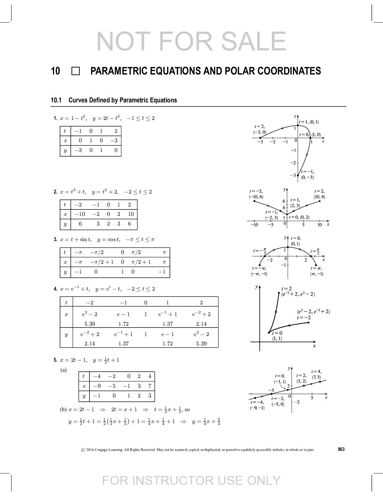
Buy this document to get the full access instantly
Instant Download Access after purchase
Add to cartInstant download
Reviews( 0 )
Document information
Connected school, study & course
About the document
Uploaded On
Jan 06, 2020
Number of pages
2
Written in

Additional information
This document has been written for:
Uploaded
Jan 06, 2020
Downloads
0
Views
103