Calculus > QUESTIONS & ANSWERS > Chapter 15: MULTIPLE INTEGRALS. Work and Answers (All)
Chapter 15: MULTIPLE INTEGRALS. Work and Answers
Document Content and Description Below
15.1 Double Integrals over Rectangles 1. (a) The subrectangles are shown in the figure. The surface is the graph of ( ) = and ∆ = 4, so we estimate ≈ 3 = 1 2... = 1 ( )∆ = (2 2)∆ + (24)∆ + (42)∆ + (44)∆ + (62)∆ + (6 4)∆ = 4(4) + 8(4) + 8(4) + 16(4) + 12(4) + 24(4) = 288 (b) ≈ 3 = 1 2 = 1 ∆ = (1 1)∆ + (13)∆ + (3 1)∆ + (33)∆ + (51)∆ + (5 3)∆ = 1(4) + 3(4) + 3(4) + 9(4) + 5(4) + 15(4) = 144 2. (a) The subrectangles are shown in the figure. Here ∆ = 2 and we estimate 1 − 2 ≈ 2 = 1 3 = 1 ∗ ∗ ∆ = (2 −1)∆ + (20)∆ + (2 1)∆ + (4 −1)∆ + (40)∆ + (41)∆ = (−1)(2) + 1(2) + (−1)(2) + (−3)(2) + 1(2) + (−3)(2) = −12 (b) 1 − 2 ≈ 2 = 1 3 = 1 ∗ ∗ ∆ = (00)∆ + (01)∆ + (02)∆ + (2 0)∆ + (21)∆ + (22)∆ = 1(2) + 1(2) + 1(2) + 1(2) + (−1)(2) + (−7)(2) = −8 3. (a) The subrectangles are shown in the figure. Since ∆ = 1 · 1 2 = 1 2, we estimate − ≈ 2 =1 2 =1 ∗ ∗ ∆ = 1 1 2 ∆ + (11)∆ + 2 1 2 ∆ + (2 1)∆ = −12 1 2 + −1 1 2 + 2−1 1 2 + 2−2 1 2 ≈ 0990 (b) − ≈ 2 =1 2 =1 ( )∆ = 1 2 1 4 ∆ + 1 2 3 4 ∆ + 3 2 1 4 ∆ + 3 2 3 4 ∆ = 1 2 −18 1 2 + 1 2 −38 1 2 + 3 2 −38 1 2 + 3 2 −98 1 2 ≈ 1151 °c 2016 Cengage Learning. All Rights Reserved. May not be scanned, copied, or duplicated, or posted to a publicly accessible website, in whole or in part. 523 NOT FOR SALE INSTRUCTOR USE ONLY © Cengage Learning. All Rights Reserved.524 ¤ CHAPTER 15 MULTIPLE INTEGRALS 4. (a) The subrectangles are shown in the figure. The surface is the graph of ( ) = 1 + 2 + 3 and ∆ = 1 2 · 3 2 = 3 4, so we estimate = (1 + 2 + 3) ≈ 2 =1 2 =1 ∗ ∗ ∆ = (10)∆ + 1 3 2 ∆ + 3 2 0 ∆ + 3 2 3 2 ∆ = 2 3 4 + 13 2 3 4 + 13 4 3 4 + 31 4 3 4 = 39 2 3 4 = 117 8 = 14625 (b) = (1 + 2 + 3) ≈ 2 =1 2 =1 ( )∆ = 5 4 3 4 ∆ + 5 4 9 4 ∆ + 7 4 3 4 ∆ + 7 4 9 4 ∆ = 77 16 3 4 + 149 16 3 4 + 101 16 3 4 + 173 16 3 4 = 375 16 = 234375 5. The values of ( ) = 52 − 2 − 2 get smaller as we move farther from the origin, so on any of the subrectangles in the problem, the function will have its largest value at the lower left corner of the subrectangle and its smallest value at the upper right corner, and any other value will lie between these two. So using these subrectangles we have . (Note that this is true no matter how is divided into subrectangles.) 6. To approximate the volume, let be the planar region corresponding to the surface of the water in the pool, and place on coordinate axes so that and correspond to the dimensions given. Then we define ( ) to be the depth of the water at ( ), so the volume of water in the pool is the volume of the solid that lies above the rectangle = [020] × [0 30] and below the graph of ( ). We can estimate this volume using the Midpoint Rule with = 2 and = 3, so ∆ = 100. Each subrectangle with its midpoint is shown in the figure. Then ≈ 2 = 1 3 = 1 ∆ = ∆[(55) + (5 15) + (525) + (15 5) + (1515) + (1525)] = 100(3 + 7 + 10 + 3 + 5 + 8) = 3600 Thus, we estimate that the pool contains 3600 cubic feet of water. Alternatively, we can approximate the volume with a Riemann sum where = 4, = 6 and the sample points are taken to be, for example, the upper right corner of each subrectangle. Then ∆ = 25 and ≈ 4 = 1 6 = 1 ( )∆ = 25[3 + 4 + 7 + 8 + 10 + 8 + 4 + 6 + 8 + 10 + 12 + 10 + 3 + 4 + 5 + 6 + 8 + 7 + 2 + 2 + 2 + 3 + 4 + 4] = 25(140) = 3500 So we estimate that the pool contains 3500 ft3 of water. °c 2016 Cengage Learning. All Rights Reserved. May not be scanned, copied, or duplicated, or posted to a publicly accessible website, in whole or in part. NOT FOR SALE INSTRUCTOR USE ONLY © Cengage Learning. All Rights Reserved.SECTION 15.1 DOUBLE INTEGRALS OVER RECTANGLES ¤ 525 7. (a) With = = 2, we have ∆ = 4. Using the contour map to estimate the value of at the center of each subrectangle, we have ( ) ≈ 2 = 1 2 = 1 ∆ = ∆[(11) + (13) + (31) + (3 3)] ≈ 4(27 + 4 + 14 + 17) = 248 (b) ave = (1) ( ) ≈ 16 1 (248) = 155 8. As in Example 9, we place the origin at the southwest corner of the state. Then = [0 388] × [0276] (in miles) is the rectangle corresponding to Colorado and we define ( ) to be the temperature at the location ( ). The average temperature is given by ave = 1 () ( ) = 388 1· 276 ( ) To use the Midpoint Rule with = = 4, we divide into 16 regions of equal size, as shown in the figure, with the center of each subrectangle indicated. The area of each subrectangle is ∆ = 388 4 · 276 4 = 6693, so using the contour map to estimate the function values at each midpoint, we have ( ) ≈ 4 = 1 4 = 1 ∆ ≈ ∆[31 + 28 + 52 + 43 + 43 + 25 + 57 + 46 + 36 + 20 + 42 + 45 + 30 + 23 + 43 + 41] = 6693(605) Therefore, ave ≈ 6693 · 605 388 · 276 ≈ 378, so the average temperature in Colorado at 4:00 PM on February 26, 2007, was approximately 378◦F. 9. = √2 0, so we can interpret the double integral as the volume of the solid that lies below the plane = √2 and above the rectangle [26] × [−15]. is a rectangular solid, so √2 = 4 · 6 · √2 = 24√2. °c 2016 Cengage Learning. All Rights Reserved. May not be scanned, copied, or duplicated, or posted to a publicly accessible website, in whole or in part. NOT FOR SALE INSTRUCTOR USE ONLY © Cengage Learning. All Rights Reserved.526 ¤ CHAPTER 15 MULTIPLE INTEGRALS 10. = 2 + 1 ≥ 0 for 0 ≤ ≤ 2, so we can interpret the integral as the volume of the solid that lies below the plane = 2 + 1 and above the rectangle [02] × [0 4]. We can picture as a rectangular solid (with height 1) surmounted by a triangular cylinder; thus (2 + 1) = (2)(4)(1) + 1 2(2)(4)(4) = 24 11. = 4 − 2 ≥ 0 for 0 ≤ ≤ 1, so we can interpret the integral as the volume of the solid that lies below the plane = 4 − 2 and above the square [01] × [01]. We can picture as a rectangular solid (with height 2) surmounted by a triangular cylinder; thus (4 − 2) = (1)(1)(2) + 1 2(1)(1)(2) = 3 12. Here = 9 − 2, so 2 + 2 = 9, ≥ 0. Thus the integral represents the volume of the top half of the part of the circular cylinder 2 + 2 = 9 that lies above the rectangle [04] × [02]. 13. 02( + 322) = 22 + 3 33 2 =2 =0 = 1 2 2 + 32 =2 =0 = 1 2(2)2 + (2)32 − 1 2(0)2 + (0)32 = 2 + 82, 03( + 322) = + 32 33 =3 =0 = + 23 =3 =0 = (3) + 2(3)3 − (0) + 2(0)3 = 3 + 272 14. 02 √ + 2 = · 2 3( + 2)32 =2 =0 = 2 3 (4)32 − 2 3 (2)32 = 16 3 − 4 3√2 = 4 3(4 − √2), 03 √ + 2 = 22 √ + 2 =3 =0 = 1 2(3)2√ + 2 − 1 2(0)2√ + 2 = 9 2√ + 2 15. 14 02(62 − 2) = 14 322 − 2 =2 =0 = 14 122 − 4 − (0 − 0) = 14(122 − 4) = 43 − 224 1 = (256 − 32) − (4 − 2) = 222 16. 01 01 ( + )2 = 01 01 (2 + 2 + 2) = 01 1 3 3 + 2 + 2 =1 =0 = 01( 1 3 + + 2) = 1 3 + 1 2 2 + 1 3 31 0 = 1 3 + 1 2 + 1 3 − 0 = 7 6 17. 01 12( + −) = 01 1 2 2 + − =2 =1 = 01 (2 + 2−) − ( 1 2 + −) = 01( 3 2 + −) = 3 2 − −1 0 = 3 2 − −1 − (0 − 1) = 5 2 − −1 °c 2016 Cengage Learning. All Rights Reserved. May not be scanned, copied, or duplicated, or posted to a publicly accessible website, in whole or in part. NOT FOR SALE INSTRUCTOR USE ONLY © Cengage Learning. All Rights Reserved.SECTION 15.1 DOUBLE INTEGRALS OVER RECTANGLES ¤ 527 18. 06 02(sin + sin) = 06 [ sin − cos] = =02 = 06 2 sin − 0 − (0 − 1) = 06 2 sin + 1 = − 2 cos + 0 6 = − 2 · √23 + 6 − − 2 + 0 = 2 3 − √43 19. −33 02( + 2 cos) = −33 + 2 sin = =02 = −33 2 + 2 = 4 2 + 1 333 −3 = 94 + 9 − 94 − 9 = 18 20. 13 15 ln = 13 1 15 ln [by Equation 11] = [ln||]3 1 1 2(ln)25 1 [substitute = ln ⇒ = (1)] = (ln 3 − 0) · 1 2[(ln 5)2 − 0] = 1 2(ln 3)(ln 5)2 21. 14 12 + = 14 ln|| + 1 · 12 2 =2 =1 = 14 ln 2 + 23 = 1 22 ln 2 + 3 2 ln|| 4 1 = 8ln2 + 3 2 ln 4 − 1 2 ln 2 + 0 = 15 2 ln 2 + 3 2 ln 4 or 15 2 ln 2 + 3 ln(412) = 21 2 ln 2 22. 0102 − = 0102 − = 02 01 − [by Equation 11] = []2 0 (− − 1)−1 0 [by integrating by parts] = 2 − 0−2−1 − −0 = (2 − 1)(1 − 2−1) or 2 − 2 + 2−1 − 1 23. 0302 2 sin3 = 02 sin3 03 2 [by Equation 11] = 02(1 − cos2)sin 03 2 = 1 3 cos3 − cos 0 2 1 333 0 = (0 − 0) − 1 3 − 1· 1 3 (27 − 0) = 2 3(9) = 6 24. 0101 2 + 2 = 01 1 3(2 + 2)32 =1 =0 = 1 3 01 [(2 + 1)32 − 3] = 1 3 01[(2 + 1)32 − 4] = 1 3 1 5(2 + 1)52 − 1 551 0 = 15 1 (252 − 1) − (1 − 0) = 15 2 2√2 − 1 25. 01 01 ( + 2)4 = 01 1 5( + 2)5 =1 =0 = 1 5 01 (1 + 2)5 − (0 + 2)5 = 1 5 01 (1 + 2)5 − 11 = 1 5 1 2 · 1 6(1 + 2)6 − 12 1 121 0 [substitute = 1 + 2 ⇒ = 2 in the first term] = 1 60 (26 − 1) − (1 − 0) = 60 1 (63 − 1) = 31 30 26. 0101 √ + = 01 2 3( + )32 =1 =0 = 2 3 01[(1 + )32 − 32] = 2 3 2 5(1 + )52 − 2 5521 0 = 4 15[(252 − 1) − (1 − 0)] = 15 4 252 − 2 or 15 8 2√2 − 1 27. sec2 = 02 04 sec2 = 02 04 sec2 = 1 222 0 tan 0 4 = (2 − 0) (tan 4 − tan 0) = 2(1 − 0) = 2 °c 2016 Cengage Learning. All Rights Reserved. May not be scanned, copied, or duplicated, or posted to a publicly accessible website, in whole or in part. NOT FOR SALE INSTRUCTOR USE ONLY © Cengage Learning. All Rights Reserved.528 ¤ CHAPTER 15 MULTIPLE INTEGRALS 28. ( + −2) = 12 02( + −2) = 12 + 1 2 2−2 =2 =0 = 12 2 + 2−2 = 2 − 2−12 1 = (4 − 1) − (1 − 2) = 4 29. 2+ 1 2 = 01 −33 2+ 1 2 = 01 2+ 1 −33 2 = 1 2 ln(2 + 1)1 0 1 3 33 −3 = 1 2 (ln 2 − ln 1) · 1 3(27 + 27) = 9 ln 2 30. √tan 1 −2 = 012 03 √tan 1 −2 = 012 √11− 2 03 tan = sin−1 1 02 ln|sec| 0 3 = sin−1 1 2 − sin−1 0 ln sec 3 − ln|sec 0| = 6 − 0(ln 2 − ln 1) = 6 ln 2 31. 0603 sin( + ) = 06 −cos( + ) = = 03 = 06 cos − cos + 3 = sin − sin + 3 0 6 − 06 sin − sin + 3 [by integrating by parts separately for each term] = 6 1 2 − 1 − −cos + cos + 3 0 6 = − 12 − − √23 + 0 − −1 + 1 2 = √32−1 − 12 32. 1 + = 01 01 1 + = 01 ln(1 + ) =1 =0 = 01 ln(1 + ) − ln 1 = 01 ln(1 + ) = (1 + )ln(1 + ) − 1 0 [by integrating by parts] = (2 ln 2 − 1) − (ln 1 − 0) = 2 ln 2 − 1 33. − = 03 02 − = 03 −− =2 =0 = 03(−−2 + 1) = 1 2 −2 + 3 0 = 1 2 −6 + 3 − 1 2 + 0 = 1 2 −6 + 5 2 34. 1 + 1 + = 13 12 1 + 1 + = 13 [ln(1 + + )] =2 =1 = 13 [ln( + 3) − ln( + 2)] = ( + 3) ln( + 3) − ( + 3) − ( + 2) ln( + 2) − ( + 2) 3 1 [by integrating by parts separately for each term] = (6 ln 6 − 6 − 5ln5 + 5) − (4 ln 4 − 4 − 3ln3 + 3) = 6ln6 − 5ln5 − 4ln4 + 3 ln 3 35. = ( ) = 4 − − 2 ≥ 0 for 0 ≤ ≤ 1 and 0 ≤ ≤ 1. So the solid is the region in the first octant which lies below the plane = 4 − − 2 and above [0 1] × [0 1]. °c 2016 Cengage Learning. All Rights Reserved. May not be scanned, copied, or duplicated, or posted to a publicly accessible website, in whole or in part. NOT FOR SALE INSTRUCTOR USE ONLY © Cengage Learning. All Rights Reserved.SECTION 15.1 DOUBLE INTEGRALS OVER RECTANGLES ¤ 529 36. = 2 − 2 − 2 ≥ 0 for 0 ≤ ≤ 1 and 0 ≤ ≤ 1. So the solid is the region in the first octant which lies below the circular paraboloid = 2 − 2 − 2 and above [01] × [01]. 37. The solid lies under the plane 4 + 6 − 2 + 15 = 0 or = 2 + 3 + 15 2 so = (2 + 3 + 15 2 ) = −11 −21(2 + 3 + 15 2 ) = −11 2 + 3 + 15 2 =2 =−1 = −11 (19 + 6) − (− 13 2 − 3) = −11( 51 2 + 9) = 51 2 + 9 2 21 −1 = 30 − (−21) = 51 38. = (32 − 2 + 2) = −11 12(32 − 2 + 2) = −11 3 − 2 + 2 =2 =1 = −11 (12 − 22) − (3 − 2) = −11 9 − 2 = 9 − 1 3 31 −1 = 26 3 + 26 3 = 52 3 39. = −22 −11 1 − 1 4 2 − 1 9 2 = 40201 1 − 1 4 2 − 1 9 2 = 402 − 12 1 3 − 1 9 2 = 1 = 0 = 402 11 12 − 1 9 2 = 4 11 12 − 27 1 32 0 = 4 · 83 54 = 166 27 40. The solid lies under the surface = 2 + 2 and above the rectangle = [0 5] × [−22], so its volume is = (2 + 2) = 05 −22(2 + 2) = 05 2 + 1 3 3 =2 =−2 = 05 22 + 8 3 − −22 − 8 3 = 05(42 + 16 3 ) = 4 3 3 + 8 3 25 0 = 500 3 + 200 3 − 0 = 700 3 41. The solid lies under the surface = 1 + 2 and above the rectangle = [−11] × [01], so its volume is = (1 + 2) = 01 −11(1 + 2) = 01 + 1 3 3 =1 =−1 = 01(2 + 2 3 ) = 2 + 2 3 ( − 1)1 0 [by integrating by parts in the second term] = (2 + 0) − 0 − 2 3 0 = 2 + 2 3 = 8 3 42. The cylinder intersects the -plane along the line = 4, so in the first octant, the solid lies below the surface = 16 − 2 and above the rectangle = [0 4] × [0 5] in the -plane. = 0504(16 − 2) = 04(16 − 2) 05 = 16 − 1 3 34 0 5 0 = (64 − 64 3 − 0)(5 − 0) = 640 3 43. The solid lies below the surface = 2 + 2 + ( − 2)2 and above the plane = 1 for −1 ≤ ≤ 1, 0 ≤ ≤ 4. The volume of the solid is the difference in volumes between the solid that lies under = 2 + 2 + ( − 2)2 over the rectangle °c 2016 Cengage Learning. All Rights Reserved. May not be scanned, copied, or duplicated, or posted to a publicly accessible website, in whole or in part. NOT FOR SALE INSTRUCTOR USE ONLY © Cengage Learning. All Rights Reserved.530 ¤ CHAPTER 15 MULTIPLE INTEGRALS = [−11] × [04] and the solid that lies under = 1 over . = 04−11[2 + 2 + ( − 2)2] − 04−11(1) = 04 2 + 1 33 + ( − 2)2 = 1 = −1 − −11 04 = 04 (2 + 1 3 + ( − 2)2) − (−2 − 1 3 − ( − 2)2) − []1 −1 []4 0 = 04 14 3 + 2( − 2)2 − [1 − (−1)][4 − 0] = 14 3 + 2 3( − 2)34 0 − (2)(4) = 56 3 + 16 3 − 0 − 16 3 − 8 = 88 3 − 8 = 64 3 44. The solid lies below the plane = + 2 and above the surface = 2 2 + 1 for 0 ≤ ≤ 2, 0 ≤ ≤ 4. The volume of the solid is the difference in volumes between the solid that lies under = + 2 over the rectangle = [02] × [04] and the solid that lies under = 2 2 + 1 over . = 02 04( + 2) − 02 04 22 + 1 = 02 + 2 =4 =0 − 02 22+ 1 04 = 02 [(4 + 16) − (0 + 0)] − ln 2 + 1 2 0 1 224 0 = 22 + 162 0 − (ln 5 − ln 1) (8 − 0) = (8 + 32 − 0) − 8ln5 = 40 − 8ln5 45. In Maple, we can calculate the integral by defining the integrand as f and then using the command int(int(f,x=0..1),y=0..1);. In Mathematica, we can use the command Integrate[f,{x,0,1},{y,0,1}] We find that 53 = 21 − 57 ≈ 00839. We can use plot3d (in Maple) or Plot3D (in Mathematica) to graph the function. 46. In Maple, we can calculate the integral by defining f:=exp(-xˆ2)*cos(xˆ2+yˆ2); and g:=2-xˆ2-yˆ2; and then [since 2 − 2 − 2 −2cos(2 + 2) for −1 ≤ ≤ 1, −1 ≤ ≤ 1] using the command evalf(Int(Int(g-f,x=-1..1),y=-1..1));. Using Int rather than int forces Maple to use purely numerical techniques in evaluating the integral. In Mathematica, we can use the command NIntegrate[g-f,{x,-1,1},{y,-1,1}]. We find that (2 − 2 − 2) − −2cos(2 + 2) ≈ 30271. We can use the plot3d command (in Maple) or Plot3D (in Mathematica) to graph both functions on the same screen. °c 2016 Cengage Learning. All Rights Reserved. May not be scanned, copied, or duplicated, or posted to a publicly accessible website, in whole or in part. NOT FOR SALE INSTRUCTOR USE ONLY © Cengage Learning. All Rights Reserved.SECTION 15.1 DOUBLE INTEGRALS OVER RECTANGLES ¤ 531 47. is the rectangle [−11] × [05]. Thus, () = 2 · 5 = 10 and ave = 1 () ( ) = 10 1 05−11 2 = 10 1 05 1 33 = 1 = −1 = 10 1 05 2 3 = 10 1 1 325 0 = 5 6. 48. () = 4 · 1 = 4, so ave = 1 () ( ) = 1 4 04 01 √ + = 1 4 04 2 3( + )32 =1 =0 = 1 4 · 2 3 04[( + )32 − ( + 1)32] = 1 6 2 5( + )52 − 2 5( + 1)524 0 = 1 6 · 2 5 [(4 + )52 − 552 − 52 + 1] = 15 1 [(4 + )52 − 52 − 552 + 1] ≈ 3327 49. 1 +4 = −11 01 1 +4 = −11 1 +4 01 [by Equation 11] but () = 1 +4 is an odd function so −11 () = 0 (by Theorem 4.5.6 [ET 5.5.7]). Thus 1 +4 = 0 · 01 = 0. 50. (1 + 2 sin + 2 sin) = 1 + 2 sin + 2 sin = () + − − 2 sin + − − 2 sin = (2)(2) + − 2 − sin + − sin − 2 But sin is an odd function, so − sin = − sin = 0 (by Theorem 4.5.6 [ET 5.5.7]) and (1 + 2 sin + 2 sin) = 42 + 0 + 0 = 42. 51. Let ( ) = − ( + )3 . Then a CAS gives 0101 ( ) = 1 2 and 0101 ( ) = − 1 2. To explain the seeming violation of Fubini’s Theorem, note that has an infinite discontinuity at (00) and thus does not satisfy the conditions of Fubini’s Theorem. In fact, both iterated integrals involve improper integrals which diverge at their lower limits of integration. 52. (a) Loosely speaking, Fubini’s Theorem says that the order of integration of a function of two variables does not affect the value of the double integral, while Clairaut’s Theorem says that the order of differentiation of such a function does not affect the value of the second-order derivative. Also, both theorems require continuity (though Fubini’s allows a finite number of smooth curves to contain discontinuities). (b) To find , we first hold constant and use the single-variable Fundamental Theorem of Calculus, Part 1: = ( ) = ( ) = ( ). Now we use the Fundamental Theorem again: = ( ) = ( ). To find , we first use Fubini’s Theorem to find that ( ) = ( ) , and then use the Fundamental Theorem twice, as above, to get = ( ). So = = ( ). °c 2016 Cengage Learning. All Rights Reserved. May not be scanned, copied, or duplicated, or posted to a publicly accessible website, in whole or in part. NOT FOR SALE INSTRUCTOR USE ONLY © Cengage Learning. All Rights Reserved.532 ¤ CHAPTER 15 MULTIPLE INTEGRALS 15.2 Double Integrals over General Regions 1. 15 0(8 − 2) = 15 8 − 2 = =0 = 15[8() − ()2 − 8(0) + (0)2] = 15 72 = 7 335 1 = 7 3(125 − 1) = 868 3 2. 02 02 2 = 02 1 33 = =02 = 02 13 (2)3 − (0)3 = 02 1 37 = 1 3 1 882 0 = 1 3(32 − 0) = 32 3 3. 01 0 3 = 01 1 223 = =0 = 01 1 23 ()2 − (0)2 = 1 2 01 23 = 1 2 1 331 0 = 1 2 · 1 3 1 − 0 = 1 6( − 1) 4. 02 0 sin = 02 [(−cos)] = =0 = 02 (−cos + ) = 02 ( − cos ) = 1 22 − (sin + cos ) 0 2 (by integrating by parts in the second term) = 1 2 · 42 − 2 − 0 − (0 − 0 − 1) = 82 − 2 + 1 5. 01 02 cos(3) = 01 cos(3) = =02 = 01 2 cos(3) = 1 3 sin(3)1 0 = 1 3 (sin 1 − sin 0) = 1 3 sin 1 6. 01 0 √1 + = 01 √1 + = =0 = 01 √1 + = 2 3(1 + )321 0 = 2 3 (1 + )32 − 2 3(1 + 1)32 = 2 3(1 + )32 − 4 3√2 7. 2 + 1 = 04 0√ 2 + 1 = 04 21+ 1 · 22 ==0√ = 12 04 2+ 1 = 1 2 1 2 ln 2 + 1 4 0 = 1 4 ln2 + 1 4 0 = 1 4(ln 17 − ln 1) = 1 4 ln 17 8. (2 + ) = 12 1−1(2 + ) = 12 2 + =1 =−1 = 12 1 + − ( − 1)2 − ( − 1) = 12(−22 + 4) = − 2 33 + 222 1 = − 16 3 + 8 − − 2 3 + 2 = 4 3 9. −2 = 03 0 −2 = 03 −2 = =0 = 03 −2 − 0 = 03 −2 = − 1 2 −23 0 = − 1 2 −9 − 0 = 1 2 1 − −9 10. 2 − 2 = 02 0 2 − 2 = 02 − 1 3(2 − 2)32 = =0 = 02 0 + 1 3(2)32 = 02 1 33 = 1 3 · 1 442 0 = 12 1 (16 − 0) = 4 3 11. (a) At the right we sketch an example of a region that can be described as lying between the graphs of two continuous functions of (a type I region) but not as lying between graphs of two continuous functions of (a type II region). The regions shown in Figures 6 and 8 in the text are additional examples. °c 2016 Cengage Learning. All Rights Reserved. May not be scanned, copied, or duplicated, or posted to a publicly accessible website, in whole or in part. NOT FOR SALE INSTRUCTOR USE ONLY © Cengage Learning. All Rights Reserved.SECTION 15.2 DOUBLE INTEGRALS OVER GENERAL REGIONS ¤ 533 (b) Now we sketch an example of a region that can be described as lying between the graphs of two continuous functions of but not as lying between graphs of two continuous functions of . The first region shown in Figure 7 is another example. 12. (a) At the right we sketch an example of a region that can be described as lying between the graphs of two continuous functions of (a type I region) and also as lying between graphs of two continuous functions of (a type II region). For additional examples see Figures 9, 11, 12, and 14–16 in the text. (b) Now we sketch an example of a region that can’t be described as lying between the graphs of two continuous functions of or between graphs of two continuous functions of . The region shown in Figure 18 is another example. 13. As a type I region, lies between the lower boundary = 0 and the upper boundary = for 0 ≤ ≤ 1, so = {( ) | 0 ≤ ≤ 1, 0 ≤ ≤ }. If we describe as a type II region, lies between the left boundary = and the right boundary = 1 for 0 ≤ ≤ 1, so = {( ) | 0 ≤ ≤ 1, ≤ ≤ 1}. Thus = 010 = 01 = = 0 = 01 2 = 1 331 0 = 1 3(1 − 0) = 1 3 or = 011 = 01 1 22 = 1 = = 1 2 01(1 − 2) = 1 2 − 1 331 0 = 1 2 1 − 1 3 − 0 = 1 3. 14. The curves = 2 and = 3 intersect at points (00), (39). As a type I region, is enclosed by the lower boundary = 2 and the upper boundary = 3 for 0 ≤ ≤ 3, so = ( ) | 0 ≤ ≤ 3, 2 ≤ ≤ 3. If we describe as a type II region, is enclosed by the left boundary = 3 and the right boundary = √ for 0 ≤ ≤ 9, so = ( ) | 0 ≤ ≤ 9, 3 ≤ ≤ √. Thus °c 2016 Cengage Learning. All Rights Reserved. May not be scanned, copied, or duplicated, or posted to a publicly accessible website, in whole or in part. NOT FOR SALE INSTRUCTOR USE ONLY © Cengage Learning. All Rights Reserved.534 ¤ CHAPTER 15 MULTIPLE INTEGRALS = 0332 = 03 · 1 22 = 3 = 2 = 1 2 03 (92 − 4) = 1 2 03(93 − 5) = 1 2 9 · 1 44 − 1 663 0 = 1 2 9 4 · 81 − 1 6 · 729 − 0 = 243 8 or = 09 √3 = 09 1 22 = = √3 = 1 2 09 − 1 92 = 1 2 09 2 − 1 93 = 1 2 1 33 − 1 9 · 1 449 0 = 1 2 1 3 · 729 − 36 1 · 6561 − 0 = 243 8 15. The curves = − 2 or = + 2 and = 2 intersect when + 2 = 2 ⇔ 2 − − 2 = 0 ⇔ ( − 2)( + 1) = 0 ⇔ = −1, = 2, so the points of intersection are (1 −1) and (42). If we describe as a type I region, the upper boundary curve is = √ but the lower boundary curve consists of two parts, = −√ for 0 ≤ ≤ 1 and = − 2 for 1 ≤ ≤ 4. Thus = {( ) | 0 ≤ ≤ 1, − √ ≤ ≤ √ } ∪ {( ) | 1 ≤ ≤ 4, − 2 ≤ ≤ √ } and = 01−√√ + 14√−2 . If we describe as a type II region, is enclosed by the left boundary = 2 and the right boundary = + 2 for −1 ≤ ≤ 2, so = ( ) | −1 ≤ ≤ 2, 2 ≤ ≤ + 2 and = −212+2 . In either case, the resulting iterated integrals are not difficult to evaluate but the region is more simply described as a type II region, giving one iterated integral rather than a sum of two, so we evaluate the latter integral: = −212+2 = −21 = = +2 2 = −21( + 2 − 2) = −21(2 + 2 − 3) = 1 33 + 2 − 1 442 −1 = 8 3 + 4 − 4 − − 1 3 + 1 − 1 4 = 9 4 16. As a type I region, = {( ) | 0 ≤ ≤ 4, ≤ ≤ 4} and 2 = 044 2 . As a type II region, = {( ) | 0 ≤ ≤ 4, 0 ≤ ≤ } and 2 = 040 2 . Evaluating 2 requires integration by parts whereas 2 does not, so the iterated integral corresponding to as a type II region appears easier to evaluate. 2 = 04 0 2 = 04 = =0 = 04 2 − = 1 22 − 1 224 0 = 1 216 − 8 − 1 2 − 0 = 1 216 − 17 2 17. 0102 cos = 01 sin = = 02 = 01 sin2 = − 1 2 cos21 0 = − 1 2(cos 1 − cos 0) = 1 2(1 − cos 1) °c 2016 Cengage Learning. All Rights Reserved. May not be scanned, copied, or duplicated, or posted to a publicly accessible website, in whole or in part. NOT FOR SALE INSTRUCTOR USE ONLY © Cengage Learning. All Rights Reserved.SECTION 15.2 DOUBLE INTEGRALS OVER GENERAL REGIONS ¤ 535 18. (2 + 2) = 01 3(2 + 2) = 01 2 + 2 = = 3 = 01(3 + 2 − 5 − 6) = 1 44 + 1 33 − 1 66 − 1 771 0 = 1 4 + 1 3 − 1 6 − 1 7 = 23 84 19. 2 = 12 7−−13 2 = 12 2 =7 =−−31 = 12 [(7 − 3) − ( − 1)] 2 = 12(82 − 43) = 8 33 − 42 1 = 64 3 − 16 − 8 3 + 1 = 11 3 20. = 01 0√1−2 = 01 1 22 = =0√1−2 = 01 1 2(1 − 2) = 1 2 01( − 3) = 1 2 1 22 − 1 441 0 = 1 2 1 2 − 1 4 − 0 = 1 8 21. −22 −√√44−−22 (2 − ) = −22 2 − 1 22 = =√−√4−4 −22 = −22 2 √4 − 2 − 1 2 4 − 2 + 2 √4 − 2 + 1 2 4 − 2 = −22 4 √4 − 2 = − 4 3 4 − 2322 −2 = 0 [Or, note that 4√4 − 2 is an odd function, so −22 4 √4 − 2 = 0.] 22. = 01 4−3 = 01 [] =4 =−3 = 01(4 − 32 − 2) = 01(4 − 42) = 22 − 4 331 0 = 2 − 4 3 − 0 = 2 3 23. D = 01 √2(3 + 2) = 01 3 + 2 ==√ 2 = 01 (3√ + ) − (33 + 4) = 01(332 + − 33 − 4) = 3 · 2 552 + 1 22 − 3 44 − 1 551 0 = 6 5 + 1 2 − 3 4 − 1 5 − 0 = 3 4 °c 2016 Cengage Learning. All Rights Reserved. May not be scanned, copied, or duplicated, or posted to a publicly accessible website, in whole or in part. NOT FOR SALE INSTRUCTOR USE ONLY © Cengage Learning. All Rights Reserved.536 ¤ CHAPTER 15 MULTIPLE INTEGRALS 24. = −22 42(1 + 22) = −22 + 1 332 =4 =2 = −22(4 + 61 3 2 − 1 38) = 4 + 61 9 3 − 27 1 92 −2 = 8 + 488 9 − 512 27 + 8 + 488 9 − 512 27 = 2336 27 25. = 1217 − 3 = 12 1 22 = 7 = 1 − 3 = 1 2 12 (7 − 3)2 − 1 = 1 2 12(48 − 422 + 93) = 1 2 242 − 143 + 9 442 1 = 31 8 26. = 02 02−(2 + 2 + 1) = 02 2 + 1 33 + =2 =0− = 02 2(2 − ) + 1 3(2 − )3 + (2 − ) − 0 = 02 − 4 33 + 42 − 5 + 14 3 = − 1 34 + 4 33 − 5 22 + 14 3 2 0 = − 16 3 + 32 3 − 10 + 28 3 − 0 = 14 3 27. = 02 04−2(4 − 2 − ) = 02 4 − 2 − 1 22 =4 =0−2 = 02 4(4 − 2) − 2(4 − 2) − 1 2(4 − 2)2 − 0 = 02 22 − 8 + 8 = 2 33 − 42 + 82 0 = 16 3 − 16 + 16 − 0 = 16 3 28. = 01 2− = 01 =2 =− = 01(2 − 22) = 2 − 2 331 0 = 1 3 29. = −22 42 2 = −22 2 =4 =2 = −22(42 − 4) = 4 33 − 1 552 −2 = 32 3 − 32 5 + 32 3 − 32 5 = 128 15 °c 2016 Cengage Learning. All Rights Reserved. May not be scanned, copied, or duplicated, or posted to a publicly accessible website, in whole or in part. NOT FOR SALE INSTRUCTOR USE ONLY © Cengage Learning. All Rights Reserved.SECTION 15.2 DOUBLE INTEGRALS OVER GENERAL REGIONS ¤ 537 30. = 0202 4 − 2 = 02 4 − 2 = 2 = 0 = 02 2 4 − 2 = − 2 3 4 − 2322 0 = 0 + 16 3 = 16 3 31. = 01 0√1 − 2 = 01 22 = = 0√1 − 2 = 01 1 −22 = 1 2 − 1 331 0 = 1 3 32. By symmetry, the desired volume is 8 times the volume 1 in the first octant. Now 1 = 00√2 − 2 2 − 2 = 0 2 − 2 = = 0√2 − 2 = 0(2 − 2) = 2 − 1 33 0 = 2 33 Thus = 16 3 3. 33. From the graph, it appears that the two curves intersect at = 0 and at ≈ 1213. Thus the desired integral is ≈ 0121334 − 2 = 01213 = 3 = 4 − 2 = 01213(32 − 3 − 5) = 3 − 1 44 − 1 661 0213 ≈ 0713 34. The desired solid is shown in the first graph. From the second graph, we estimate that = cos intersects = at ≈ 07391. Therefore the volume of the solid is ≈ 007391cos = 007391 = cos = = 007391(cos − 2) = cos + sin − 1 330 07391 ≈ 01024 Note: There is a different solid which can also be construed to satisfy the conditions stated in the exercise. This is the solid bounded by all of the given surfaces, as well as the plane = 0. In case you calculated the volume of this solid and want to check your work, its volume is ≈ 0073910 + 0 7391 2 0cos ≈ 04684. °c 2016 Cengage Learning. All Rights Reserved. May not be scanned, copied, or duplicated, or posted to a publicly accessible website, in whole or in part. NOT FOR SALE INSTRUCTOR USE ONLY © Cengage Learning. All Rights Reserved.538 ¤ CHAPTER 15 MULTIPLE INTEGRALS 35. The region of integration is bounded by the curves = 1 − 2 and = 2 − 1 which intersect at (±1 0) with 1 − 2 ≥ 2 − 1 on [−1 1]. Within this region, the plane = 2 + 2 + 10 is above the plane = 2 − − , so = −11 12−−12(2 + 2 + 10) − −11 12−−12(2 − − ) = −11 12−−12(2 + 2 + 10 − (2 − − )) = −11 12−−12(3 + 3 + 8) = −11 3 + 3 2 2 + 8 =1 =−2−21 = −11 3(1 − 2) + 3 2(1 − 2)2 + 8(1 − 2) − 3(2 − 1) − 3 2(2 − 1)2 − 8(2 − 1) = −11(−63 − 162 + 6 + 16) = − 3 24 − 16 3 3 + 32 + 161 −1 = − 3 2 − 16 3 + 3 + 16 + 3 2 − 16 3 − 3 + 16 = 64 3 36. The two planes intersect in the line = 1, = 3, so the region of integration is the plane region enclosed by the parabola = 2 and the line = 1. We have 2 + ≥ 3 for 0 ≤ ≤ 1, so the solid region is bounded above by = 2 + and bounded below by = 3. = −11 12(2 + ) − −11 12(3) = −11 12(2 + − 3) = −11 12(2 − 2) = −11 2 − 2 =1 =2 = −11(1 − 22 + 4) = − 2 33 + 1 5 51 −1 = 16 15 37. The region of integration is bounded by the curves = 2 and = 1 − 2 which intersect at ± √12 1 2 . The solid lies under the graph of = 3 and above the graph of = , so its volume is = 1√2 −1√2 12−2 3 − −11√√22 12−2 = −11√√22 12−2(3 − ) = 1√2 −1√2 3 − 1 2 2 =1 =−2 2 = −11√√22 3(1 − 2) − 1 2(1 − 2)2 − 32 − 1 2(2)2 = 1√2 −1√2 5 2 − 52 = 5 2 − 5 3 31 −1√√2 2 = 2√5 2 − 6√5 2 − − 2√5 2 + 6√5 2 = 10 3√2 or 5√3 2 °c 2016 Cengage Learning. All Rights Reserved. May not be scanned, copied, or duplicated, or posted to a publicly accessible website, in whole or in part. NOT FOR SALE INSTRUCTOR USE ONLY © Cengage Learning. All Rights Reserved.SECTION 15.2 DOUBLE INTEGRALS OVER GENERAL REGIONS ¤ 539 38. The region of integration is the portion of the first quadrant bounded by the axes and the curve = √4 − 2. The solid lies under the graph of = + and above the graph of = , so its volume is = 02 0√4−2( + ) − 02 0√4−2 = 02 0√4−2( + − ) = 02 + 1 2 2 − 1 2 2 = =0√4−2 = 02 √4 − 2 + 1 2(4 − 2) − 1 2(4 − 2) − 0 = 02 √4 − 2 + 2 − 1 2 2 − 2 + 1 23 = − 1 3(4 − 2)32 + 2 − 1 6 3 − 2 + 1 842 0 = 4 − 4 3 − 4 + 2 − − 1 3 · 432 = 2 3 + 8 3 = 10 3 39. The solid lies below the plane = 1 − − or + + = 1 and above the region = {( ) | 0 ≤ ≤ 10 ≤ ≤ 1 − } in the -plane. The solid is a tetrahedron. 40. The solid lies below the plane = 1 − and above the region = ( ) | 0 ≤ ≤ 1 0 ≤ ≤ 1 − 2 in the -plane. 41. The two bounding curves = 3 − and = 2 + intersect at the origin and at = 2, with 2 + 3 − on (02). Using a CAS, we find that the volume of the solid is = 0232−+(34 + 2) = 1314 ,984 ,549 ,735 ,535 ,616 42. For || ≤ 1 and || ≤ 1, 22 + 2 8 − 2 − 22. Also, the cylinder is described by the inequalities −1 ≤ ≤ 1, −√1 − 2 ≤ ≤ √1 − 2. So the volume is given by = −11 −√√11−−22 (8 − 2 − 22) − (22 + 2) = 132 [using a CAS] 43. The two surfaces intersect in the circle 2 + 2 = 1, = 0 and the region of integration is the disk : 2 + 2 ≤ 1. Using a CAS, the volume is (1 − 2 − 2) = −11 −√√11−−22(1 − 2 − 2) = 2 . °c 2016 Cengage Learning. All Rights Reserved. May not be scanned, copied, or duplicated, or posted to a publicly accessible website, in whole or in part. NOT FOR SALE INSTRUCTOR USE ONLY © Cengage Learning. All Rights Reserved.540 ¤ CHAPTER 15 MULTIPLE INTEGRALS 44. The projection onto the -plane of the intersection of the two surfaces is the circle 2 + 2 = 2 ⇒ 2 + 2 − 2 = 0 ⇒ 2 + ( − 1)2 = 1, so the region of integration is given by −1 ≤ ≤ 1, 1 − √1 − 2 ≤ ≤ 1 + √1 − 2. In this region, 2 ≥ 2 + 2 so, using a CAS, the volume is = −11 1−1+√√1−1−22[2 − (2 + 2)] = 2 45. Because the region of integration is = {( ) | 0 ≤ ≤ 0 ≤ ≤ 1} = {( ) | ≤ ≤ 1 0 ≤ ≤ 1} we have 01 0 ( ) = ( ) = 01 1 ( ) . 46. Because the region of integration is = ( ) | 2 ≤ ≤ 40 ≤ ≤ 2 = ( ) | 0 ≤ ≤ √0 ≤ ≤ 4 we have 02 42 ( ) = ( ) = 04 0√ ( ) . 47. Because the region of integration is = {( ) | 0 ≤ ≤ cos0 ≤ ≤ 2} = ( ) | 0 ≤ ≤ cos−1 0 ≤ ≤ 1 we have 02 0cos ( ) = ( ) = 01 0cos−1 ( ) . 48. Because the region of integration is = ( ) | 0 ≤ ≤ 4 − 2 −2 ≤ ≤ 2 = ( ) | −√4 − 2 ≤ ≤ √4 − 20 ≤ ≤ 2 we have −22 0√4−2 ( ) = ( ) = 02 √4−2 −√4−2 ( ) . 49. Because the region of integration is = {( ) | 0 ≤ ≤ ln, 1 ≤ ≤ 2} = {( ) | ≤ ≤ 2, 0 ≤ ≤ ln 2} we have 120ln ( ) = ( ) = 0ln 22 ( ) °c 2016 Cengage Learning. All Rights Reserved. May not be scanned, copied, or duplicated, or posted to a publicly accessible website, in whole or in part. NOT FOR SALE INSTRUCTOR USE ONLY © Cengage Learning. All Rights Reserved.SECTION 15.2 DOUBLE INTEGRALS OVER GENERAL REGIONS ¤ 541 50. Because the region of integration is = ( ) | arctan ≤ ≤ 4 , 0 ≤ ≤ 1 = ( ) | 0 ≤ ≤ tan, 0 ≤ ≤ 4 we have 01arctan 4 ( ) = ( ) = 04 0tan ( ) 51. 0133 2 = 0303 2 = 03 2 = =03 = 03 32 = 1 6 23 0 = 9 6− 1 52. 0112 √ sin = 010√ √ sin = 01 √ sin [] = =0√ = 01 (√ sin)(√ − 0) = 01 sin = − cos ]1 0 + 01 cos [by integrating by parts with = , = sin ] = [− cos + sin]1 0 = −cos 1 + sin 1 − 0 = sin 1 − cos 1 53. 01√1 3 + 1 = 0102 3 + 1 = 01 3 + 1 [] = =02 = 01 23 + 1 = 2 9 3 + 1321 0 = 2 9 232 − 132 = 2 9 2√2 − 1 54. 0212 cos(3 − 1) = 0102 cos(3 − 1) = 01 cos(3 − 1) 1 22 =2 =0 = 01 22 cos(3 − 1) = 2 3 sin(3 − 1)1 0 = 2 3 [0 − sin(−1)] = − 2 3 sin(−1) = 2 3 sin 1 °c 2016 Cengage Learning. All Rights Reserved. May not be scanned, copied, or duplicated, or posted to a publicly accessible website, in whole or in part. NOT FOR SALE INSTRUCTOR USE ONLY © Cengage Learning. All Rights Reserved.542 ¤ CHAPTER 15 MULTIPLE INTEGRALS 55. 01arcsin 2 cos 1 + cos2 = 02 0sin cos √1 + cos2 = 02 cos √1 + cos2 =sin =0 = 02 cos √1 + cos2 sin Let = cos = , (−=sin − sin ) , = 10 − √1 + 2 = − 1 31 + 2320 1 = 1 3 √8 − 1 = 1 32√2 − 1 56. 08 √32 4 = 0203 4 = 02 4 = =03 = 02 34 = 1 4 42 0 = 1 4(16 − 1) 57. = {( ) | 0 ≤ ≤ 1, − + 1 ≤ ≤ 1} ∪ {( ) | −1 ≤ ≤ 0, + 1 ≤ ≤ 1} ∪ {( ) | 0 ≤ ≤ 1, − 1 ≤ ≤ − 1} ∪ {( ) | −1 ≤ ≤ 0, − 1 ≤ ≤ − − 1}, all type I. 2 = 0111− 2 + −01 1+ 1 2 + 01−1− 1 2 + −01 −−1 − 1 2 = 40111− 2 [by symmetry of the regions and because ( ) = 2 ≥ 0] = 401 3 = 4 1 441 0 = 1 58. = ( ) | −1 ≤ ≤ 0, − 1 ≤ ≤ − 3 ∪ ( ) | 0 ≤ ≤ 1, √ − 1 ≤ ≤ − 3, both type II. = −01 −1−3 + 01√−−13 = −01 = = −−13 + 01 = = √−−31 = −01(2 − 4 + ) + 01(2 − 4 − 32 + ) = 1 33 − 1 55 + 1 220 −1 + 1 33 − 1 55 − 2 552 + 1 221 0 = (0 − 11 30) + ( 30 7 − 0) = − 15 2 59. Since 2 + 2 ≤ 1 on , we must have 0 ≤ 2 ≤ 1 and 0 ≤ 2 ≤ 1, so 0 ≤ 22 ≤ 1 ⇒ 3 ≤ 4 − 22 ≤ 4 ⇒ √3 ≤ 4 − 22 ≤ 2. Here we have () = 1 2(1)2 = 2 , so by Property 11, √3() ≤ 4 − 22 ≤ 2() ⇒ √23 ≤ 4 − 22 ≤ or we can say 2720 4 − 22 3142. (We have rounded the lower bound down and the upper bound up to preserve the inequalities.) °c 2016 Cengage Learning. All Rights Reserved. May not be scanned, copied, or duplicated, or posted to a publicly accessible website, in whole or in part. NOT FOR SALE INSTRUCTOR USE ONLY © Cengage Learning. All Rights Reserved.SECTION 15.2 DOUBLE INTEGRALS OVER GENERAL REGIONS ¤ 543 60. is the triangle with vertices (0 0), (10), and (12) so () = 1 2(1)(2) = 1. We have 0 ≤ sin4( + ) ≤ 1 for all , , and Property 11 gives 0 · () ≤ sin4( + ) ≤ 1 · () ⇒ 0 ≤ sin4( + ) ≤ 1. 61. The average value of a function of two variables defined on a rectangle was defined in Section 15.1 as ave = (1) ( ). Extending this definition to general regions , we have ave = (1) ( ). Here = {( ) | 0 ≤ ≤ 1 0 ≤ ≤ 3}, so () = 1 2(1)(3) = 3 2 and ave = (1) ( ) = 312 01 03 = 2 3 01 1 22 =3 =0 = 1 3 01 93 = 3 441 0 = 3 4 62. Here = ( ) | 0 ≤ ≤ 10 ≤ ≤ 2, so () = 01 2 = 1 331 0 = 1 3 and ave = (1) ( ) = 113 01 02 sin = 301 −cos = =02 = 301 − cos(2) = 3 1 22 − 1 2 sin(2)1 0 = 3 1 2 − 1 2 sin 1 − 0 = 3 2(1 − sin 1) 63. Since ≤ ( ) ≤ , ≤ ( ) ≤ by (8) ⇒ 1 ≤ ( ) ≤ 1 by (7) ⇒ () ≤ ( ) ≤ () by (10). 64. ( ) = 0102 ( ) + 1303− ( ) = 02 3−2 ( ) 65. First we can write ( + 2) = + 2. But ( ) = is an odd function with respect to [that is, (− ) = −( )] and is symmetric with respect to . Consequently, the volume above and below the graph of is the same as the volume below and above the graph of , so = 0. Also, 2 = 2 · () = 2 · 1 2(3)2 = 9 since is a half disk of radius 3. Thus ( + 2) = 0 + 9 = 9. 66. The graph of ( ) = 2 − 2 − 2 is the top half of the sphere 2 + 2 + 2 = 2, centered at the origin with radius , and is the disk in the -plane also centered at the origin with radius . Thus 2 − 2 − 2 represents the volume of a half ball of radius which is 1 2 · 4 3 3 = 2 33. °c 2016 Cengage Learning. All Rights Reserved. May not be scanned, copied, or duplicated, or posted to a publicly accessible website, in whole or in part. NOT FOR SALE INSTRUCTOR USE ONLY © Cengage Learning. All Rights Reserved.544 ¤ CHAPTER 15 MULTIPLE INTEGRALS 67. We can write (2 + 3) = 2 + 3 . 2 represents the volume of the solid lying under the plane = 2 and above the rectangle . This solid region is a triangular cylinder with length and whose cross-section is a triangle with width and height 2. (See the first figure.) Thus its volume is 1 2 · · 2 · = 2. Similarly, 3 represents the volume of a triangular cylinder with length , triangular cross-section with width and height 3, and volume 1 2 · · 3 · = 3 22. (See the second figure.) Thus (2 + 3) = 2 + 3 22 68. In the first quadrant, and are positive and the boundary of is + = 1. But is symmetric with respect to both axes because of the absolute values, so the region of integration is the square shown at the left. To evaluate the double integral, we first write (2 + 23 − 2 sin) = 2 + 23 − 2 sin . Now ( ) = 23 is odd with respect to [that is, ( −) = −( )] and is symmetric with respect to , so 23 = 0. Similarly, ( ) = 2 sin is odd with respect to [since (− ) = −( )] and is symmetric with respect to , so 2 sin = 0. is a square with side length √2, so 2 = 2 · () = 2√22 = 4, and (2 + 23 − 2 sin) = 4 + 0 + 0 = 4. 69. 3 + 3 + √2 − 2 = 3 + 3 + √2 − 2 . Now 3 is odd with respect to and 3 is odd with respect to , and the region of integration is symmetric with respect to both and , so 3 = 3 = 0. √2 − 2 represents the volume of the solid region under the graph of = √2 − 2 and above the rectangle , namely a half circular cylinder with radius and length 2 (see the figure) whose volume is 1 2 · 2 = 1 22(2) = 2. Thus 3 + 3 + √2 − 2 = 0 + 0 + 2 = 2. °c 2016 Cengage Learning. All Rights Reserved. May not be scanned, copied, or duplicated, or posted to a publicly accessible website, in whole or in part. NOT FOR SALE INSTRUCTOR USE ONLY © Cengage Learning. All Rights Reserved.SECTION 15.3 DOUBLE INTEGRALS IN POLAR COORDINATES ¤ 545 70. To find the equations of the boundary curves, we require that the -values of the two surfaces be the same. In Maple, we use the command solve(4-xˆ2-yˆ2=1-x-y,y); and in Mathematica, we use Solve[4-xˆ2-yˆ2==1-x-y,y]. We find that the curves have equations = 1 ± √13 + 4 − 42 2 . To find the two points of intersection of these curves, we use the CAS to solve 13 + 4 − 42 = 0, finding that = 1 ± √14 2 . So, using the CAS to evaluate the integral, the volume of intersection is = (1(1 + − √√1414))22 11 + −√√13 + 4 13 + 4 −−442222[(4 − 2 − 2) − (1 − − )] = 498 15.3 Double Integrals in Polar Coordinates 1. The region is more easily described by polar coordinates: = {( ) | 2 ≤ ≤ 5, 0 ≤ ≤ 2}. Thus ( ) = 0225 ( cos sin) . 2. The region is more easily described by rectangular coordinates: = {( ) | −1 ≤ ≤ 1, − ≤ ≤ 1}. Thus ( ) = −11 −1 ( ) . 3. The region is more easily described by polar coordinates: = {( ) | 0 ≤ ≤ 1, ≤ ≤ 2}. Thus ( ) = 2 01 ( cos sin) . 4. The region is more easily described by polar coordinates: = ( ) | 0 ≤ ≤ 3, − 4 ≤ ≤ 34 . Thus ( ) = −3 44 03 ( cos sin) . 5. The integral 3 4 4 12 represents the area of the region = {( ) | 1 ≤ ≤ 2, 4 ≤ ≤ 34}, the top quarter portion of a ring (annulus). 3 4 4 12 = 3 4 4 12 = 3 44 1 2 22 1 = 34 − 4 · 1 2 (4 − 1) = 2 · 3 2 = 34 6. The integral 2 02 sin represents the area of the region = {( ) | 0 ≤ ≤ 2sin, 2 ≤ ≤ }. Since = 2 sin ⇒ 2 = 2 sin ⇔ 2 + 2 = 2 ⇔ 2 + ( − 1)2 = 1, is the portion in the second quadrant of a disk of radius 1 with center (01). 2 02 sin = 2 1 2 2 =2 sin =0 = 2 2sin2 = 2 2 · 1 2(1 − cos 2) = − 1 2 sin 2 2 = − 0 − 2 + 0 = 2 °c 2016 Cengage Learning. All Rights Reserved. May not be scanned, copied, or duplicated, or posted to a publicly accessible website, in whole or in part. NOT FOR SALE INSTRUCTOR USE ONLY © Cengage Learning. All Rights Reserved.546 ¤ CHAPTER 15 MULTIPLE INTEGRALS 7. The half disk can be described in polar coordinates as = {( ) | 0 ≤ ≤ 5, 0 ≤ ≤ }. Then 2 = 0 05 ( cos)2( sin) = 0 cos2 sin 05 4 = − 1 3 cos3 0 1 555 0 = − 1 3(−1 − 1) · 625 = 1250 3 8. The region is 1 8 of a disk, as shown in the figure, and can be described by = {( ) | 0 ≤ ≤ 2, 4 ≤ ≤ 2}. Thus (2 − ) = 42 02(2 cos − sin) = 42(2cos − sin) 02 2 = 2sin + cos 2 4 1 332 0 = (2 + 0 − √2 − √22) 8 3 = 16 3 − 4√2 9. sin(2 + 2) = 02 13 sin(2) = 02 13 sin(2) = 0 2 − 1 2 cos(2)3 1 = 2 − 1 2(cos 9 − cos 1) = 4 (cos 1 − cos 9) 10. 2 +2 2 = 02 ( sin 2)2 = 02 sin2 = 02 1 2(1 − cos 2) = 1 2 − 1 2 sin 22 0 1 22 = 1 2 (2 − 0 − 0) · 1 2 2 − 2 = 2 (2 − 2) 11. −2−2 = − 22 02 −2 = − 22 02 −2 = − 2 2 − 1 2−22 0 = − 1 2 (−4 − 0) = 2 (1 − −4) 12. cos2 + 2 = 02 02 cos√2 = 02 02 cos . For the second integral, integrate by parts with = , = cos . Then cos2 + 2 = 2 0 [ sin + cos]2 0 = 2(2 sin 2 + cos 2 − 1). 13. is the region shown in the figure, and can be described by = {( ) | 0 ≤ ≤ 41 ≤ ≤ 2}. Thus arctan() = 04 12 arctan(tan) since = tan. Also, arctan(tan) = for 0 ≤ ≤ 4, so the integral becomes 04 12 = 04 12 = 1 22 0 4 1 222 1 = 322 · 3 2 = 64 3 2. 14. = 2 + 2 ≤ 4 ≥ 0, ≥ 0 − ( − 1)2 + 2 ≤ 1 ≥ 0 = 0202 2 cos − 0202 cos 2 cos = 02 1 3(8 cos) − 02 13(8 cos4 ) = 8 3 − 8 12 cos3 sin + 3 2( + sin cos) 0 2 = 8 3 − 2 3 0 + 3 2 2 = 16 −6 3 °c 2016 Cengage Learning. All Rights Reserved. May not be scanned, copied, or duplicated, or posted to a publicly accessible website, in whole or in part. NOT FOR SALE INSTRUCTOR USE ONLY © Cengage Learning. All Rights Reserved.SECTION 15.3 DOUBLE INTEGRALS IN POLAR COORDINATES ¤ 547 15. One loop is given by the region = {( )|−6 ≤ ≤ 6, 0 ≤ ≤ cos 3 }, so the area is = − 66 0cos 3 = − 66 1 22 =cos 3 =0 = − 66 1 2 cos2 3 = 206 1 21 + cos6 2 = 1 2 + 16 sin6 0 6 = 12 16. By symmetry, the area of the region is 4 times the area of the region in the first quadrant enclosed by the cardiod = 1 − cos (see the figure). Here = {( ) | 0 ≤ ≤ 1 − cos 0 ≤ ≤ 2}, so the total area is 4() = 4 = 402 01−cos = 402 1 22 =1 =0−cos = 202(1 − cos)2 = 202(1 − 2cos + cos2 ) = 202 1 − 2cos + 1 2(1 + cos2) = 2 − 2sin + 1 2 + 1 4 sin2 0 2 = 2 2 − 2 + 4 = 32 − 4 17. In polar coordinates the circle ( − 1)2 + 2 = 1 ⇔ 2 + 2 = 2 is 2 = 2 cos ⇒ = 2cos, and the circle 2 + 2 = 1 is = 1. The curves intersect in the first quadrant when 2cos = 1 ⇒ cos = 1 2 ⇒ = 3, so the portion of the region in the first quadrant is given by = {( ) | 1 ≤ ≤ 2cos0 ≤ ≤ 3}. By symmetry, the total area is twice the area of : 2() = 2 = 203 12 cos = 203 1 22 =2 cos =1 = 03 4cos2 − 1 = 03 4 · 1 2(1 + cos2) − 1 = 03(1 + 2cos2) = [ + sin2] 0 3 = 3 + √23 18. The region lies between the two polar curves in quadrants I and IV, but in quadrants II and III the region is enclosed by the cardioid. In the first quadrant, 1 + cos = 3cos when cos = 1 2 ⇒ = 3 , so the area of the region inside the cardioid and outside the circle is 1 = 32 3 cos 1+cos = 32 1 22 =1+cos =3 cos = 1 2 32(1 + 2cos − 8cos2 ) = 1 2 + 2sin − 8 1 2 + 1 4 sin2 2 3 = − 3 2 + sin − sin2 2 3 = − 34 + 1 − 0 − − 2 + √23 − √23 = 1 − 4 [continued] °c 2016 Cengage Learning. All Rights Reserved. May not be scanned, copied, or duplicated, or posted to a publicly accessible website, in whole or in part. NOT FOR SALE INSTRUCTOR USE ONLY © Cengage Learning. All Rights Reserved.548 ¤ CHAPTER 15 MULTIPLE INTEGRALS The area of the region in the second quadrant is 2 = 2 01+cos = 2 1 22 =1+cos =0 = 1 2 2(1 + 2 cos + cos2 ) = 1 2 + 2 sin + 1 2 + 1 4 sin 2 2 = 1 2 34 − 2 = 38 − 1 By symmetry, the total area is = 2(1 + 2) = 21 − 4 + 38 − 1 = 4 . 19. = 2 + 2 ≤25 2 + 2 = 0205 2 · = 02 05 3 = 2 0 1 445 0 = 2 625 4 = 625 2 20. = 1 ≤ 2 + 2 ≤4 2 + 2 = 0212 √2 = 02 12 2 = 2 0 1 332 1 = 2 8 3 − 1 3 = 14 3 21. 2 + + = 4 ⇔ = 4 − 2 − , so the volume of the solid is = 2 + 2 ≤1 (4 − 2 − ) = 0201(4 − 2 cos − sin) = 0201 4 − 2 (2 cos + sin) = 0222 − 1 33 (2 cos + sin) =1 =0 = 022 − 1 3 (2 cos + sin) = 2 − 1 3 (2 sin − cos)2 0 = 4 + 1 3 − 0 − 1 3 = 4 22. The sphere 2 + 2 + 2 = 16 intersects the -plane in the circle 2 + 2 = 16, so = 2 4≤2+2≤16 16 − 2 − 2 [by symmetry] = 20224 16 − 2 = 202 24 (16 − 2)12 = 2 2 0 − 1 3(16 − 2)324 2 = − 2 3(2)(0 − 1232) = 43 12√12 = 32√3 23. By symmetry, = 2 2 + 2 ≤ 2 2 − 2 − 2 = 2020 2 − 2 = 202 0 2 − 2 = 2 2 0 − 1 3(2 − 2)32 0 = 2(2)0 + 1 33 = 4 33 24. The paraboloid = 1 + 22 + 22 intersects the plane = 7 when 7 = 1 + 22 + 22 or 2 + 2 = 3 and we are restricted to the first octant, so = 2+2 ≤ 3 ≥0≥0 7 − 1 + 22 + 22 = 020√3 7 − (1 + 22) = 02 0√3 6 − 23 = 0 2 32 − 1 24√ 0 3 = 2 · 9 2 = 9 4 25. The cone = 2 + 2 intersects the sphere 2 + 2 + 2 = 1 when 2 + 2 + 2 + 2 2 = 1 or 2 + 2 = 1 2. So = 2 + 2 ≤ 12 1 − 2 − 2 − 2 + 2 = 0201√2 1 − 2 − = 02 01√2 √1 − 2 − 2 = 2 0 − 1 3(1 − 2)32 − 1 331 0√2 = 2− 1 3 √12 − 1 = 3 2 − √2 °c 2016 Cengage Learning. All Rights Reserved. May not be scanned, copied, or duplicated, or posted to a publicly accessible website, in whole or in part. NOT FOR SALE INSTRUCTOR USE ONLY © Cengage Learning. All Rights Reserved.SECTION 15.3 DOUBLE INTEGRALS IN POLAR COORDINATES ¤ 549 26. The two paraboloids intersect when 6 − 2 − 2 = 22 + 22 or 2 + 2 = 2. For 2 + 2 ≤ 2, the paraboloid = 6 − 2 − 2 is above = 22 + 22 so = 2 + 2 ≤ 2 [(6 − 2 − 2) − (22 + 22)] = 2 + 2 ≤ 2 [6 − 3(2 + 2)] = 020√2(6 − 32) = 02 0√2(6 − 33) = 2 0 32 − 3 44√ 0 2 = 2 (6 − 3) = 6 27. The given solid is the region inside the cylinder 2 + 2 = 4 between the surfaces = 64 − 42 − 42 and = −64 − 42 − 42. So = 2 + 2 ≤ 4 64 − 42 − 42 − −64 − 42 − 42 = 2+2 ≤ 4 2 · 216 − 2 − 2 = 40202 √16 − 2 = 402 02 √16 − 2 = 4 2 0 − 1 3(16 − 2)322 0 = 8− 1 3(1232 − 1623) = 83 64 − 24√3 28. (a) Here the region in the -plane is the annular region 12 ≤ 2 + 2 ≤ 22 and the desired volume is twice that above the -plane. Hence = 2 2 1 ≤ 2 + 2 ≤ 22 22 − 2 − 2 = 20212 22 − 2 = 202 12 22 − 2 = 2 (2)− 1 3(22 − 2)32 2 1 = 43(22 − 12)32 (b) A cross-sectional cut is shown in the figure. So 22 = 1 22 + 12 or 1 4 2 = 22 − 12. Thus the volume in terms of is = 4 3 1 4232 = 6 3. 29. 020√4−2 −2−2 = 02 02 −2 = 02 02 −2 = 0 2 − 1 2−22 0 = 2 − 1 2 −4 − 1 = 4 1 − −4 30. 0−√√22−−22 (2 + ) = 0 0(2 cos + sin) = 0(2 cos + sin) 0 2 = [2 sin − cos] 0 1 33 0 = [(0 + 1) − (0 − 1)] · 1 3(3 − 0) = 2 33 °c 2016 Cengage Learning. All Rights Reserved. May not be scanned, copied, or duplicated, or posted to a publicly accessible website, in whole or in part. NOT FOR SALE INSTRUCTOR USE ONLY © Cengage Learning. All Rights Reserved.550 ¤ CHAPTER 15 MULTIPLE INTEGRALS 31. The region of integration is shown in the figure. In polar coordinates the line = √3 is = 6, so 012√√3 1−2 2 = 06 01( cos)( sin)2 = 06 sin2 cos 01 4 = 1 3 sin3 0 6 1 551 0 = 1 3 1 23 − 0 1 5 − 0 = 120 1 32. 0202 cos 2 = 02 1 33 =2 cos =0 = 02 8 3 cos3 = 8 3 02 (1 − sin2 )cos = 8 3 sin − 1 3 sin3 0 2 = 16 9 33. = {( ) | 0 ≤ ≤ 1, 0 ≤ ≤ 2}, so (2+2)2 = 02 01 (2)2 = 02 01 4 = 201 4 . Using a calculator, we estimate 201 4 ≈ 45951. 34. = {( ) | 0 ≤ ≤ 1, 0 ≤ ≤ 2}, so 1 + 2 + 2 = 02 01 ( cos)( sin)√1 + 2 = 02 sin cos 01 3√1 + 2 = 1 2 sin2 0 2 01 3√1 + 2 = 1 2 01 3√1 + 2 ≈ 01609 35. The surface of the water in the pool is a circular disk with radius 20 ft. If we place on coordinate axes with the origin at the center of and define ( ) to be the depth of the water at ( ), then the volume of water in the pool is the volume of the solid that lies above = ( ) | 2 + 2 ≤ 400 and below the graph of ( ). We can associate north with the positive -direction, so we are given that the depth is constant in the -direction and the depth increases linearly in the -direction from (0 −20) = 2 to (020) = 7. The trace in the -plane is a line segment from (0 −20 2) to (0207). The slope of this line is 20 −7 −(−220) = 1 8, so an equation of the line is − 7 = 1 8( − 20) ⇒ = 1 8 + 9 2. Since ( ) is independent of , ( ) = 1 8 + 9 2. Thus the volume is given by ( ), which is most conveniently evaluated using polar coordinates. Then = {( ) | 0 ≤ ≤ 20, 0 ≤ ≤ 2} and substituting = cos, = sin the integral becomes 02020 1 8 sin + 9 2 = 02 24 1 3 sin + 9 42 = 20 = 0 = 02 1000 3 sin + 900 = − 1000 3 cos + 9002 0 = 1800 Thus the pool contains 1800 ≈ 5655 ft3 of water. °c 2016 Cengage Learning. All Rights Reserved. May not be scanned, copied, or duplicated, or posted to a publicly accessible website, in whole or in part. NOT FOR SALE INSTRUCTOR USE ONLY © Cengage Learning. All Rights Reserved.SECTION 15.3 DOUBLE INTEGRALS IN POLAR COORDINATES ¤ 551 36. (a) If ≤ 100, the total amount of water supplied each hour to the region within feet of the sprinkler is = 020 − = 02 0 − = 2 0 −− − − 0 = 2[−− − − + 0 + 1] = 2(1 − − − −) ft3 (b) The average amount of water per hour per square foot supplied to the region within feet of the sprinkler is area of region = 2 = 21 − − − − 2 ft3 (per hour per square foot). See the definition of the average value of a function on page 1037 [ET 997]. 37. As in Exercise 15.2.61, ave = (1) ( ). Here = {( ) | ≤ ≤ 0 ≤ ≤ 2}, so () = 2 − 2 = ( 2 − 2) and ave = 1 () 21+ 2 = ( 21− 2) 02 √12 = ( 21− 2) 02 = 1 ( 2 − 2) 2 0 = 1 ( 2 − 2) (2)( − ) = ( +2()( −−) ) = +2 38. The distance from a point ( ) to the origin is ( ) = 2 + 2, so the average distance from points in to the origin is ave = (1) 2 + 2 = 12 02 0 √2 = 1 2 02 0 2 = 12 []2 0 1 33 0 = 12 · 2 · 1 33 = 2 3 39. 11√2 √1 − 2 + 1√20 + √22 0√4 − 2 = 0412 3 cos sin = 04 44 cos sin = 2 = 1 = 15 4 04 sin cos = 15 4 sin22 0 4 = 15 16 40. (a) −(2+2) = 020 −2 = 2− 1 2−2 0 = 1 − −2 for each . Then lim →∞ 1 − −2 = since −2 → 0 as → ∞. Hence −∞ ∞ −∞ ∞ −(2+2) = . (b) −(2+2) = −− −2−2 = − −2 − −2 for each . Then, from (a), = R2 −(2 + 2), so = lim →∞ −(2+2) = lim →∞ − −2 − −2 = −∞ ∞ −2 −∞ ∞ −2 To evaluate lim →∞ − −2 − −2 , we are using the fact that these integrals are bounded. This is true since on [−11], 0 −2 ≤ 1 while on (−∞ −1), 0 −2 ≤ and on (1 ∞), 0 −2 −. Hence 0 ≤ −∞ ∞ −2 ≤ −∞ −1 + −11 + 1∞ − = 2(−1 + 1). °c 2016 Cengage Learning. All Rights Reserved. May not be scanned, copied, or duplicated, or posted to a publicly accessible website, in whole or in part. NOT FOR SALE INSTRUCTOR USE ONLY © Cengage Learning. All Rights Reserved.552 ¤ CHAPTER 15 MULTIPLE INTEGRALS (c) Since −∞ ∞ −2 −∞ ∞ −2 = and can be replaced by , −∞ ∞ −2 2 = implies that −∞ ∞ −2 = ±√. But −2 ≥ 0 for all , so −∞ ∞ −2 = √. (d) Letting = √2, −∞ ∞ −2 = −∞ ∞ √12 −22 , so that √ = √12 −∞ ∞ −22 or −∞ ∞ −22 = √2. 41. (a) We integrate by parts with = and = −2 . Then = and = − 1 2 −2, so 0∞ 2−2 = lim →∞ 0 2−2 = lim →∞ − 1 2 −2 0 + 0 1 2 −2 = lim →∞ − 1 2 −2 + 1 2 0∞ −2 = 0 + 1 2 0∞ −2 [by l’Hospital’s Rule] = 1 4 −∞ ∞ −2 [since −2 is an even function] = 1 4 √ [by Exercise 40(c)] (b) Let = √. Then 2 = ⇒ = 2 ⇒ 0∞ √ − = lim →∞ 0 √ − = lim →∞ 0√ −22 = 20∞ 2−2 = 2 1 4√ [by part(a)] = 1 2√. 15.4 Applications of Double Integrals 1. = ( ) = 05 25 (2 + 4) = 05 2 + 22 =5 =2 = 05 (10 + 50 − 4 − 8) = 05 (6 + 42) = 32 + 425 0 = 75 + 210 = 285 C 2. = ( ) = 2 + 2 = 02 01 √2 = 02 01 2 = []2 0 1 3 31 0 = 2 · 1 3 = 23 C 3. = ( ) = 13 14 2 = 13 14 2 = []3 1 1 3 34 1 = (2)(21) = 42, = 1 ( ) = 421 13 14 2 = 42 1 13 14 2 = 42 1 1 2 23 1 1 3 34 1 = 42 1 (4)(21) = 2, = 1 ( ) = 421 13 14 3 = 42 1 13 14 3 = 42 1 []3 1 1 4 44 1 = 42 1 (2) 255 4 = 85 28 Hence = 42, ( ) = 2 85 28. 4. = ( ) = 0 0(1 + 2 + 2) = 0 + 2 + 1 3 3 = =0 = 0 + 2 + 1 3 3 = + 1 3 3 + 1 3 3 0 = + 1 3 3 + 1 3 3 = 1 3 (3 + 2 + 2), = ( ) = 0 0( + 3 + 2) = 0 + 3 + 1 3 3 = =0 = 0 + 3 + 1 3 3 = 1 2 2 + 1 4 4 + 1 6 32 0 = 1 2 2 + 1 4 4 + 1 6 23 = 12 1 2(6 + 32 + 22), and = ( ) = 0 0( + 2 + 3) = 0 1 2 2 + 1 2 22 + 1 4 4 = =0 = 0 1 2 2 + 1 2 22 + 1 4 4 = 1 2 2 + 1 6 23 + 1 4 4 0 = 1 2 2 + 1 6 32 + 1 4 4 = 12 1 2(6 + 22 + 32). °c 2016 Cengage Learning. All Rights Reserved. May not be scanned, copied, or duplicated, or posted to a publicly accessible website, in whole or in part. NOT FOR SALE INSTRUCTOR USE ONLY © Cengage Learning. All Rights Reserved.SECTION 15.4 APPLICATIONS OF DOUBLE INTEGRALS ¤ 553 Hence, ( ) = = 12 1 1 3 2 (6 + 3 (3 + 22++ 2 2)2) 12 1 1 3 2(6 + 2 (3 + 22++ 3 2)2) = 4(3 + (6 + 322 ++ 2 2)2) (6 + 2 4(3 + 22 + 3 + 2)2) . 5. = 02 3−2( + ) = 02 + 1 22 =3 = −2 = 02 (3 − ) + 1 2(3 − )2 − 1 22 − 1 82 = 02 − 9 82 + 9 2 = − 9 8 1 33 + 9 22 0 = 6, = 02 3−2(2 + ) = 02 2 + 1 22 =3 = −2 = 02 9 2 − 9 83 = 9 2, = 02 3−2( + 2) = 02 1 22 + 1 33 =3 = −2 = 02 9 − 9 2 = 9. Hence = 6, ( ) = = 34 32. 6. Here = ( ) | 0 ≤ ≤ 2 5 2 ≤ ≤ 1 − 2. = 025 1−22 = 025 1 22 =1 = −22 = 1 2 025 (1 − 2)2 − 1 22 = 1 2 025 15 4 2 − 4 + 1 = 1 2 5 43 − 22 + 2 05 = 1 2 25 2 − 25 8 + 2 5 = 25 2 , = 025 1−22 · = 025 1 33 =1 = −22 = 1 3 025 (1 − 2)3 − 1 23 = 1 3 025 − 65 8 3 + 122 − 6 + 1 = 1 3 − 65 324 + 43 − 32 + 2 05 = 1 3 − 250 13 + 125 32 − 12 25 + 2 5 = 750 31 , = 025 1−22 · = 025 1 22 =1 = −22 = 1 2 025 15 4 2 − 4 + 1 = 1 2 025 15 4 3 − 42 + = 1 2 15 164 − 4 33 + 1 222 05 = 1 2 125 3 − 375 32 + 25 2 = 750 7 . Hence = 2 25, ( ) = 31 2 750 25 72750 25 = 31 60 60 7 . 7. = −11 01−2 = −11 1 22 =1 =0−2 = 1 2 −11(1 − 2)2 = 1 2 −11(1 − 22 + 4) = 1 2 − 2 33 + 1 551 −1 = 1 2 1 − 2 3 + 1 5 + 1 − 2 3 + 1 5 = 15 8 , = −11 01−2 = −11 1 22 =1 =0−2 = 1 2 −11 (1 − 2)2 = 1 2 −11( − 23 + 5) = 1 2 1 22 − 1 24 + 1 661 −1 = 1 2 1 2 − 1 2 + 1 6 − 1 2 + 1 2 − 1 6 = 0, = −11 01−2 2 = −11 1 33 =1 =0−2 = 1 3 −11(1 − 2)3 = 1 3 −11(1 − 32 + 34 − 6) = 1 3 − 3 + 3 55 − 1 771 −1 = 1 3 1 − 1 + 3 5 − 1 7 + 1 − 1 + 3 5 − 1 7 = 105 32 . Hence = 8 15, ( ) = 0 32 8 105 15 = 0 4 7. 8. The boundary curves intersect when + 2 = 2 ⇔ 2 − − 2 = 0 ⇔ = −1, = 2. Thus here = ( ) | −1 ≤ ≤ 2 2 ≤ ≤ + 2. = −21 2+2 2 = −21 2 = = +2 2 = −21(3 + 22 − 4) = 1 44 + 2 33 − 1 552 −1 = 44 15 + 13 60 = 63 20, °c 2016 Cengage Learning. All Rights Reserved. May not be scanned, copied, or duplicated, or posted to a publicly accessible website, in whole or in part. NOT FOR SALE INSTRUCTOR USE ONLY © Cengage Learning. All Rights Reserved.554 ¤ CHAPTER 15 MULTIPLE INTEGRALS = −21 2+2 3 = −21 3 = = +2 2 = −21(4 + 23 − 5) = 1 55 + 1 24 − 1 662 −1 = 56 15 − 15 2 = 18 5 , = −21 2+2 2 = −21 2 1 22 = = +2 2 = 1 2 −21 2 (2 + 4 + 4 − 4) = 1 2 −21(4 + 43 + 42 − 6) = 1 2 1 55 + 4 + 4 33 − 1 772 −1 = 1 2 1552 105 + 105 41 = 531 70 . Hence = 63 20, ( ) = 63 18 20 5 531 63 20 70 = 8 7 118 49 . 9. = 01 0− = 01 1 22 = =0− = 1 2 01 −2 = 1 2 01 −2 integrate by parts with = = −2 = 1 2 − 1 4(2 + 1)−21 0 = − 1 8 3−2 − 1 = 1 8 − 3 8−2, = 01 0− 2 = 01 2 1 22 = =0− = 1 2 01 2−2 [integrate by parts twice] = 1 2 − 1 4 22 + 2 + 1−21 0 = − 1 8 5−2 − 1 = 1 8 − 5 8−2, = 01 0− 2 = 01 1 33 = =0− = 1 3 01 −3 = 1 3 − 1 9(3 + 1)−31 0 = − 27 1 4−3 − 1 = 27 1 − 27 4 −3. Hence = 1 8 1 − 3−2, ( ) = 1 81 8 (11 − − 5 3 − −2 2 ) 27 11 8 (1 1−−34−−23) = 2 2 − − 5 3 27 ( 833 −− 43). 10. Note that cos ≥ 0 for −2 ≤ ≤ 2. = − 22 0cos = − 22 1 22 =cos =0 = 1 2 − 22 cos2 = 1 2 1 2 + 1 4 sin 2 − 2 2 = 4 , = − 22 0cos = − 22 1 22 =cos =0 = 1 2 − 22 cos2 integrate by parts with = = cos2 = 1 2 1 2 + 1 4 sin 2 − 2 2 − − 22 1 2 + 1 4 sin 2 = 1 2 1 82 − 1 82 − 1 42 − 1 8 cos 2 − 2 2 = 1 2 0 − 16 1 2 + 1 8 − 16 1 2 − 1 8 = 0, = − 22 0cos 2 = − 22 1 33 =cos =0 = 1 3 − 22 cos3 = 1 3 − 22(1 − sin2)cos [substitute = sin ⇒ = cos ] = 1 3 sin − 1 3 sin3 − 2 2 = 1 3 1 − 1 3 + 1 − 1 3 = 4 9 . Hence = 4 , ( ) = 0 494 = 0 916 . 11. ( ) = , = = 0201 ( sin) = 02 sin 01 2 = −cos 0 2 1 331 0 = (1) 1 3 = 1 3, = · = 0201 ( cos)( sin) = 02 sin cos 01 3 = 1 2 sin2 0 2 1 441 0 = 1 2 1 4 = 1 8, °c 2016 Cengage Learning. All Rights Reserved. May not be scanned, copied, or duplicated, or posted to a publicly accessible website, in whole or in part. NOT FOR SALE INSTRUCTOR USE ONLY © Cengage Learning. All Rights Reserved.SECTION 15.4 APPLICATIONS OF DOUBLE INTEGRALS ¤ 555 = · = 0201 ( sin)2 = 02 sin2 01 3 = 1 2 − 1 4 sin 2 0 2 1 441 0 = 4 1 4 = 16 . Hence ( ) = 8 3 316 = 3 8 316 . 12. ( ) = (2 + 2) = 2, = 0201 3 = 8 , = 0201 4 cos = 1 5 02 cos = 1 5sin 0 2 = 1 5, = 0201 4 sin = 1 5 02 sin = 1 5−cos 0 2 = 1 5. Hence ( ) = 58 58 . 13. ( ) = 2 + 2 = , = ( ) = 012 · = 0 12 2 = () 1 332 1 = 7 3, = ( ) = 012( cos)() = 0 cos 12 3 = sin 0 1 442 1 = (0) 15 4 = 0 [this is to be expected as the region and density function are symmetric about the y-axis] = ( ) = 012( sin)() = 0 sin 12 3 = −cos 0 1 442 1 = (1 + 1) 15 4 = 15 2 Hence ( ) = 0 715 23 = 0 14 45 . 14. Now ( ) = 2 + 2 = , so = ( ) = 012() = 0 12 = ()(1) = , = ( ) = 012( cos)() = 0 cos 12 = sin 0 1 222 1 = (0) 3 2 = 0, = ( ) = 012( sin)() = 0 sin 12 = −cos 0 1 222 1 = (1 + 1) 3 2 = 3. Hence ( ) = 0 3 = 0 3 . 15. Placing the vertex opposite the hypotenuse at (00), ( ) = (2 + 2). Then = 00 − 2 + 2 = 0 2 − 3 + 1 3 ( − )3 = 1 33 − 1 44 − 12 1 ( − )4 0 = 1 64. [continued] °c 2016 Cengage Learning. All Rights Reserved. May not be scanned, copied, or duplicated, or posted to a publicly accessible website, in whole or in part. NOT FOR SALE INSTRUCTOR USE ONLY © Cengage Learning. All Rights Reserved.556 ¤ CHAPTER 15 MULTIPLE INTEGRALS By symmetry, = = 00 − (2 + 2) = 0 1 2( − )22 + 1 4( − )4 = 1 623 − 1 44 + 10 1 5 − 20 1 ( − )5 0 = 15 1 5 Hence ( ) = 2 5 2 5. 16. ( ) = 2 + 2 = . = 5 6 612 sin = 5 6 6[(2 sin) − 1] = −2cos − 5 66 = 2√3 − 3 By symmetry of and () = , = 0, and = 5 6 612 sin sin = 1 2 5 6 6(4 sin3 − sin) = 1 2 −3cos + 4 3 cos3 5 66 = √3 Hence ( ) = 0 2(3 3√√3 3− ). 17. = 2( ) = 13 14 2 · 2 = 13 14 4 = []3 1 1 554 1 = (2) 1023 5 = 4092, = 2( ) = 13 14 2 · 2 = 13 2 14 2 = 1 333 1 1 334 1 = 26 3 (21) = 182, and 0 = + = 4092 + 182 = 5912. 18. = 2( ) = 025 1−22 2 · = 025 2 1 22 =1 = −22 = 1 2 025 2( 15 4 2 − 4 + 1) = 1 2 025( 15 4 4 − 43 + 2) = 1 2 3 45 − 4 + 1 332 05 = 9375 16 , = 2( ) = 025 1−22 2 · = 025 1 44 =1 = −22 = 1 4 025 (1 − 2)4 − 16 1 4 = 1 4 025( 255 16 4 − 323 + 242 − 8 + 1) = 1 4 51 165 − 84 + 83 − 42 + 2 05 = 3125 78 , and 0 = + = 9375 16 + 3125 78 = 75 2 . 19. As in Exercise 15, we place the vertex opposite the hypotenuse at (0 0) and the equal sides along the positive axes. = 00− 2(2 + 2) = 00−(22 + 4) = 0 1 323 + 1 55 = =0− = 0 1 32( − )3 + 1 5( − )5 = 1 3 1 333 − 3 424 + 3 55 − 1 66 − 30 1 ( − )6 0 = 180 7 6, = 00− 2(2 + 2) = 00−(4 + 22) = 04 + 1 323 = =0− = 04 ( − ) + 1 32 ( − )3 = 1 55 − 1 66 + 1 3 1 333 − 3 424 + 3 55 − 1 66 0 = 180 7 6, and 0 = + = 90 7 6. °c 2016 Cengage Learning. All Rights Reserved. May not be scanned, copied, or duplicated, or posted to a publicly accessible website, in whole or in part. NOT FOR SALE INSTRUCTOR USE ONLY © Cengage Learning. All Rights Reserved.SECTION 15.4 APPLICATIONS OF DOUBLE INTEGRALS ¤ 557 20. If we find the moments of inertia about the - and -axes, we can determine in which direction rotation will be more difficult. (See the explanation following Example 4.) The moment of inertia about the -axis is given by = 2( ) = 0202 2(1 + 01) = 02(1 + 01) 1 33 = 2 = 0 = 8 3 02(1 + 01) = 8 3 + 01 · 1 222 0 = 8 3(22) ≈ 587 Similarly, the moment of inertia about the -axis is given by = 2( ) = 0202 2(1 + 01) = 02 2(1 + 01) = 2 = 0 = 202(2 + 013) = 2 1 33 + 01 · 1 442 0 = 2 8 3 + 04 ≈ 613 Since , more force is required to rotate the fan blade about the -axis. 21. = 2( ) = 00 2 = 0 0 2 = 0 1 33 0 = 1 33 = 1 33, = 2( ) = 00 2 = 0 2 0 = 1 33 0 [] 0 = 1 33, and = (area of rectangle) = since the lamina is homogeneous. Hence 2 = = 1 3 3 = 2 3 ⇒ = √ 3 and 2 = = 1 3 3 = 2 3 ⇒ = √3 . 22. Here we assume 0, 0 but note that we arrive at the same results if 0 or 0. We have = ( ) | 0 ≤ ≤ 0 ≤ ≤ − , so = 00− 2 = 0 1 33 = =0− = 1 3 0 − 3 = 1 3 − 1 4 − 4 0 = − 12(0 − 4) = 12 1 3, = 00− 2 = 0 2 − = 02 − 3 = 3 3 − 44 0 = ( 33 − 43 ) = 12 1 3, and = 00− = 0 − = − 22 0 = 1 2. Hence 2 = = 1 123 1 2 = 2 6 ⇒ = √ 6 and 2 = = 1 123 1 2 = 2 6 ⇒ = √6 . 23. In polar coordinates, the region is = ( ) | 0 ≤ ≤ 0 ≤ ≤ 2 , so = 2 = 020 ( sin)2 = 02 sin2 0 3 = 1 2 − 1 4 sin 2 0 2 1 44 0 = 4 1 44 = 16 1 4, = 2 = 020 ( cos)2 = 02 cos2 0 3 = 1 2 + 1 4 sin 2 0 2 1 44 0 = 4 1 44 = 16 1 4, and = · () = · 1 42 since the lamina is homogeneous. Hence 2 = 2 = 1 164 1 4 2 = 2 4 ⇒ = = 2 . °c 2016 Cengage Learning. All Rights Reserved. May not be scanned, copied, or duplicated, or posted to a publicly accessible website, in whole or in part. NOT FOR SALE INSTRUCTOR USE ONLY © Cengage Learning. All Rights Reserved.558 ¤ CHAPTER 15 MULTIPLE INTEGRALS 24. = 00sin = 0 sin = −cos 0 = 2, = 00sin 2 = 1 3 0 sin3 = 1 3 0(1 − cos2 )sin = 1 3−cos + 1 3 cos3 0 = 4 9, = 00sin 2 = 0 2 sin = −2 cos + 2sin + 2 cos 0 [by integrating by parts twice] = (2 − 4). Then 2 = = 2 9 , so = √2 3 and 2 = = 2 − 4 2 , so = 22− 4. 25. The right loop of the curve is given by = {( ) | 0 ≤ ≤ cos 2, −4 ≤ ≤ 4}. Using a CAS, we find = ( ) = (2 + 2) = − 44 0cos 2 2 = 364 . Then = 1 ( ) = 364 − 44 0cos 2( cos)2 = 364 − 44 0cos 2 4 cos = 16384 10395√2 and = 1 ( ) = 364 − 44 0cos 2( sin)2 = 364 − 44 0cos 2 4 sin = 0, so ( ) = 16384 10395√2 0. The moments of inertia are = 2( ) = − 44 0cos 2( sin)2 2 = − 44 0cos 2 5 sin2 = 384 5 − 105 4 , = 2( ) = − 44 0cos 2( cos)2 2 = − 44 0cos 2 5 cos2 = 384 5 + 105 4 , and 0 = + = 5 192 . 26. Using a CAS, we find = ( ) = 02 0− 22 = 729 8 (5 − 899−6). Then = 1 ( ) = 8(5 −729 899−6) 02 0− 32 = 2(55 6 6 − − 1223) 899 and = 1 ( ) = 8(5 −729 899−6) 02 0− 23 = 729(45 32768(5 6 −642037 − 899) −2), so ( ) = 2(55 6 6 − − 1223) 899 729(45 32768(5 6 −642037 − 899) −2). The moments of inertia are = 2( ) = 02 0− 24 = 390625 16 (63 − 305593−10), = 2( ) = 02 0− 42 = 2187 80 (7 − 2101−6), and 0 = + = 854296875 16 (13809656 − 4103515625−6 − 668331891−10). 27. (a) ( ) is a joint density function, so we know R2 ( ) = 1. Since ( ) = 0 outside the rectangle [01] × [02], we can say R2 ( ) = −∞ ∞ −∞ ∞ ( ) = 0102 (1 + ) = 01 + 1 22 =2 =0 = 01 4 = 221 0 = 2 Then 2 = 1 ⇒ = 1 2 . °c 2016 Cengage Learning. All Rights Reserved. May not be scanned, copied, or duplicated, or posted to a publicly accessible website, in whole or in part. NOT FOR SALE INSTRUCTOR USE ONLY © Cengage Learning. All Rights Reserved.SECTION 15.4 APPLICATIONS OF DOUBLE INTEGRALS ¤ 559 (b) ( ≤ 1 ≤ 1) = −∞ 1 −∞ 1 ( ) = 0101 1 2(1 + ) = 01 12 + 1 2 2 = 1 = 0 = 01 12 3 2 = 3 4 1 2 21 0 = 3 8 or 0375 (c) ( + ≤ 1) = (( ) ∈ ) where is the triangular region shown in the figure. Thus ( + ≤ 1) = ( ) = 0101 − 1 2 (1 + ) = 01 12 + 1 2 2 = 1 = 0− = 01 1 2 1 22 − 2 + 3 2 = 1 4 01 3 − 42 + 3 = 1 4 44 − 4 33 + 3 22 1 0 = 5 48 ≈ 01042 28. (a) ( ) ≥ 0, so is a joint density function if R2 ( ) = 1. Here, ( ) = 0 outside the square [01] × [01], so R2 ( ) = 0101 4 = 01 22 = 1 = 0 = 01 2 = 21 0 = 1. Thus, ( ) is a joint density function. (b) (i) No restriction is placed on , so ≥ 1 2 = 1∞2 −∞ ∞ ( ) = 112 01 4 = 112 22 = 1 = 0 = 112 2 = 21 12 = 3 4. (ii) ≥ 1 2 ≤ 1 2 = 1∞2 −∞ 12 ( ) = 112 012 4 = 112 22 = 1 = 02 = 112 1 2 = 1 2 · 1 2 21 12 = 16 3 (c) The expected value of is given by 1 = R2 ( ) = 0101 (4) = 01 222 = 1 = 0 = 201 2 = 2 1 3 31 0 = 2 3 The expected value of is 2 = R2 ( ) = 0101 (4) = 01 4 1 33 = 1 = 0 = 4 3 01 = 4 3 1 2 21 0 = 2 3 29. (a) ( ) ≥ 0, so is a joint density function if R2 ( ) = 1. Here, ( ) = 0 outside the first quadrant, so R2 ( ) = 0∞ 0∞ 01−(05 + 02) = 010∞0∞ −05−02 = 010∞ −05 0∞ −02 = 01 lim →∞ 0 −05 lim →∞ 0 −02 = 01 lim →∞ −2−05 0 lim →∞ −5−02 0 = 01 lim →∞ −2(−05 − 1) lim →∞ −5(−02 − 1) = (01) · (−2)(0 − 1) · (−5)(0 − 1) = 1 Thus ( ) is a joint density function. (b) (i) No restriction is placed on , so ( ≥ 1) = −∞ ∞ 1∞ ( ) = 0∞1∞ 01−(05+02) = 010∞ −05 1∞ −02 = 01 lim →∞ 0 −05 lim →∞ 1 −02 = 01 lim →∞ −2−05 0 lim →∞ −5−02 1 = 01 lim →∞ −2(−05 − 1) lim →∞ −5(−02 − −02) (01) · (−2)(0 − 1) · (−5)(0 − −02) = −02 ≈ 08187 °c 2016 Cengage Learning. All Rights Reserved. May not be scanned, copied, or duplicated, or posted to a publicly accessible website, in whole or in part. NOT FOR SALE INSTRUCTOR USE ONLY © Cengage Learning. All Rights Reserved.560 ¤ CHAPTER 15 MULTIPLE INTEGRALS (ii) ( ≤ 2 ≤ 4) = −∞ 2 −∞ 4 ( ) = 0204 01−(05+02) = 0102 −05 04 −02 = 01−2−052 0 −5−024 0 = (01) · (−2)(−1 − 1) · (−5)(−08 − 1) = (−1 − 1)(−08 − 1) = 1 + −18 − −08 − −1 ≈ 03481 (c) The expected value of is given by 1 = R2 ( ) = 0∞0∞ 01−(05+02) = 010∞ −05 0∞ −02 = 01 lim →∞ 0 −05 lim →∞ 0 −02 To evaluate the first integral, we integrate by parts with = and = −05 (or we can use Formula 96 in the Table of Integrals): −05 = −2−05 − −2−05 = −2−05 − 4−05 = −2( + 2)−05. Thus 1 = 01 lim →∞ −2( + 2)−05 0 lim →∞ −5−02 0 = 01 lim →∞ (−2)( + 2)−05 − 2 lim →∞ (−5)−02 − 1 = 01(−2)lim →∞ 0+ 2 5 − 2(−5)(−1) = 2 [by l’Hospital’s Rule] The expected value of is given by 2 = R2 ( ) = 0∞0∞ 01−(05 +02) = 010∞ −05 0∞ −02 = 01 lim →∞ 0 −05 lim →∞ 0 −02 To evaluate the second integral, we integrate by parts with = and = −02 (or again we can use Formula 96 in the Table of Integrals) which gives −02 = −5−02 + 5−02 = −5( + 5)−02. Then 2 = 01 lim →∞ −2−05 0 lim →∞ −5( + 5)−02 0 = 01 lim →∞ −2(−05 − 1) lim →∞ −5( + 5)−02 − 5 = 01(−2)(−1) · (−5)lim →∞ 0+ 5 2 − 5 = 5 [by l’Hospital’s Rule] 30. (a) The lifetime of each bulb has exponential density function () = 01000 1 −1000 if if ≥ 00 If and are the lifetimes of the individual bulbs, then and are independent, so the joint density function is the product of the individual density functions: ( ) = 10 0 −6−(+)1000 if otherwise ≥ 0, ≥ 0 °c 2016 Cengage Learning. All Rights Reserved. May not be scanned, copied, or duplicated, or posted to a publicly accessible website, in whole or in part. NOT FOR SALE INSTRUCTOR USE ONLY © Cengage Learning. All Rights Reserved.SECTION 15.4 APPLICATIONS OF DOUBLE INTEGRALS ¤ 561 The probability that both of the bulbs fail within 1000 hours is ( ≤ 1000 ≤ 1000) = −∞ 1000 −∞ 1000 ( ) = 01000 01000 10−6−(+)1000 = 10−6 01000 −1000 01000 −1000 = 10−6 −1000−10001000 0 −1000−10001000 0 = −1 − 12 ≈ 03996 (b) Now we are asked for the probability that the combined lifetimes of both bulbs is 1000 hours or less. Thus we want to find ( + ≤ 1000), or equivalently (( ) ∈ ) where is the triangular region shown in the figure. Then ( + ≤ 1000) = ( ) = 01000 01000− 10−6−(+)1000 = 10−6 01000 −1000−(+)1000 =1000 =0 − = −10−3 01000 −1 − −1000 = −10−3 −1 + 1000−10001000 0 = 1 − 2−1 ≈ 02642 31. (a) The random variables and are normally distributed with 1 = 45, 2 = 20, 1 = 05, and 2 = 01. The individual density functions for and , then, are 1() = 1 05√2 −(−45)205 and 2 () = 1 01√2 −(−20)2002. Since and are independent, the joint density function is the product ( ) = 1()2() = 1 05√2 −(−45)205 011√2 −(−20)2002 = 10 −2(−45)2−50(−20)2 Then (40 ≤ ≤ 50, 20 ≤ ≤ 25) = 40 5020 25 ( ) = 10 40 5020 25 −2(−45)2−50(−20)2 . Using a CAS or calculator to evaluate the integral, we get (40 ≤ ≤ 50, 20 ≤ ≤ 25) ≈ 0500. (b) (4( − 45)2 + 100( − 20)2 ≤ 2) = 10 −2(−45)2−50(−20)2 , where is the region enclosed by the ellipse 4( − 45)2 + 100( − 20)2 = 2. Solving for gives = 20 ± 10 1 2 − 4( − 45)2, the upper and lower halves of the ellipse, and these two halves meet where = 20 [since the ellipse is centered at (45 20)] ⇒ 4( − 45)2 = 2 ⇒ = 45 ± √12. Thus 10 −2(−45)2−50(−20)2 = 10 4545+1 −1√√22 2020+ − 10 110 1√√22−−4(4( −−45) 45) 22 −2(−45)2−50(−20)2 . Using a CAS or calculator to evaluate the integral, we get (4( − 45)2 + 100( − 20)2 ≤ 2) ≈ 0632. °c 2016 Cengage Learning. All Rights Reserved. May not be scanned, copied, or duplicated, or posted to a publicly accessible website, in whole or in part. NOT FOR SALE INSTRUCTOR USE ONLY © Cengage Learning. All Rights Reserved.562 ¤ CHAPTER 15 MULTIPLE INTEGRALS 32. Because and are independent, the joint density function for Xavier’s and Yolanda’s arrival times is the product of the individual density functions: ( ) = 1()2() = 050 1 − if otherwise ≥ 0, 0 ≤ ≤ 10 Since Xavier won’t wait for Yolanda, they won’t meet unless ≥ . Additionally, Yolanda will wait up to half an hour but no longer, so they won’t meet unless − ≤ 30. Thus the probability that they meet is (( ) ∈ ) where is the parallelogram shown in the figure. The integral is simpler to evaluate if we consider as a type II region, so (( ) ∈ ) = ( ) = 010+30 50 1 − = 1 50 010 −− = = +30 = 50 1 010 (−−(+30) + −) = 1 50(1 − −30)010 − By integration by parts (or Formula 96 in the Table of Integrals), this is 1 50(1 − −30)−( + 1)−10 0 = 50 1 (1 − −30)(1 − 11−10) ≈ 0020. Thus there is only about a 2% chance they will meet. Such is student life! 33. (a) If ( ) is the probability that an individual at will be infected by an individual at , and is the number of infected individuals in an element of area , then ( ) is the number of infections that should result from exposure of the individual at to infected people in the element of area . Integration over gives the number of infections of the person at due to all the infected people in . In rectangular coordinates (with the origin at the city’s center), the exposure of a person at is = ( ) = 20 1 [20 − ( )] = 1 − 20 1 ( − 0)2 + ( − 0)2 (b) If = (00), then = 1 − 20 1 2 + 2 = 02010 1 − 20 1 = 2 1 22 − 60 1 310 0 = 250 − 50 3 = 200 3 ≈ 209 For at the edge of the city, it is convenient to use a polar coordinate system centered at . Then the polar equation for the circular boundary of the city becomes = 20 cos instead of = 10, and the distance from to a point in the city °c 2016 Cengage Learning. All Rights Reserved. May not be scanned, copied, or duplicated, or posted to a publicly accessible website, in whole or in part. NOT FOR SALE INSTRUCTOR USE ONLY © Cengage Learning. All Rights Reserved.SECTION 15.5 SURFACE AREA ¤ 563 is again (see the figure). So = − 22 020 cos 1 − 20 1 = − 22 1 2 2 − 60 1 3 =20 cos =0 = − 22 200 cos2 − 400 3 cos3 = 200 − 22 1 2 + 1 2 cos 2 − 2 31 − sin2 cos = 200 1 2 + 1 4 sin 2 − 2 3 sin + 2 3 · 1 3 sin3 − 2 2 = 200 4 + 0 − 2 3 + 2 9 + 4 + 0 − 2 3 + 2 9 = 200 2 − 8 9 ≈ 136 Therefore the risk of infection is much lower at the edge of the city than in the middle, so it is better to live at the edge. 15.5 Surface Area 1. Here = ( ) = 5 + 3 + 6 and is the rectangle [14] × [26], so by Formula 2 the area of the surface is () = [( )]2 + [( )]2 + 1 = √52 + 32 + 1 = √35 = √35() = √35 (3)(4) = 12√35 2. = ( ) = 1 2 − 3 − 2 and is the disk 2 + 2 ≤ 25, so by Formula 2 () = (−3)2 + (−2)2 + 1 = √14 = √14() = √14 ( · 52) = 25√14 3. The surface is given by = ( ) = 6 − 3 − 2 which intersects the -plane in the line 3 + 2 = 6, so is the triangular region given by ( ) 0 ≤ ≤ 2, 0 ≤ ≤ 3 − 3 2 . By Formula 2, the surface area of is () = (−3)2 + (−2)2 + 1 = √14 = √14() = √14 1 2 · 2 · 3 = 3√14 4. = ( ) = 1 4 2 − 1 2 + 5 4, and is the triangular region given by {( ) | 0 ≤ ≤ 2 0 ≤ ≤ 2}. By Formula 2, () = 1 2 2 + − 1 22 + 1 = 02 02 1 4 2 + 5 4 = 02 1 2√2 + 5 =2 =0 = 1 2 02 2 √2 + 5 = 1 2 · 2 3(2 + 5)322 0 = 1 3(932 − 532) = 9 − 5 3√5 5. The paraboloid intersects the plane = −2 when 1 − 2 − 2 = −2 ⇔ 2 + 2 = 3, so = ( ) | 2 + 2 ≤ 3. Here = ( ) = 1 − 2 − 2 ⇒ = −2, = −2 and () = (−2)2 + (−2)2 + 1 = 4(2 + 2) + 1 = 020√3 √42 + 1 = 02 0√3 √42 + 1 = 2 0 12 1 (42 + 1)32√ 0 3 = 2 · 12 1 1332 − 1 = 6 13√13 − 1 6. 2 + 2 = 4 ⇒ = √4 − 2 (since ≥ 0), so = −(4 − 2)−12, = 0 and () = 0101 [−(4 − 2)−12]2 + 02 + 1 = 0101 4 −22 + 1 = 01 √4 2− 2 01 = 2sin−1 21 0 1 0 = 2 · 6 − 0(1) = 3 °c 2016 Cengage Learning. All Rights Reserved. May not be scanned, copied, or duplicated, or posted to a publicly accessible website, in whole or in part. NOT FOR SALE INSTRUCTOR USE ONLY © Cengage Learning. All Rights Reserved.564 ¤ CHAPTER 15 MULTIPLE INTEGRALS 7. = ( ) = 2 − 2 with 1 ≤ 2 + 2 ≤ 4. Then () = 42 + 42 + 1 = 0212 √42 + 1 = 02 12 √42 + 1 = 2 0 12 1(42 + 1)322 1 = 6 17√17 − 5√5 8. = ( ) = 2 3(32 + 32) and = {( )|0 ≤ ≤ 1 0 ≤ ≤ 1}. Then = 12, = 12 and () = √ 2 + (√ )2 + 1 = 01 01 + + 1 = 01 2 3( + + 1)32 =1 =0 = 2 3 01 ( + 2)32 − ( + 1)32 = 2 3 2 5( + 2)52 − 2 5( + 1)521 0 = 4 15(352 − 252 − 252 + 1) = 15 4 (352 − 272 + 1) 9. = ( ) = with 2 + 2 ≤ 1, so = , = ⇒ () = 2 + 2 + 1 = 0201 √2 + 1 = 02 1 3(2 + 1)32 =1 =0 = 02 1 3 2√2 − 1 = 232√2 − 1 10. Given the sphere 2 + 2 + 2 = 4, when = 1, we get 2 + 2 = 3 so = ( ) | 2 + 2 ≤ 3 and = ( ) = 4 − 2 − 2. Thus () = [(−)(4 − 2 − 2)−12]2 + [(−)(4 − 2 − 2)−12]2 + 1 = 020√3 4 −22 + 1 = 020√3 2 4+ 4 − −2 2 = 020√3 √42− 2 = 02 −2(4 − 2)12==0√3 = 02(−2 + 4) = 22 0 = 4 11. = 2 − 2 − 2, = −(2 − 2 − 2)−12, = −(2 − 2 − 2)−12, () = 2 −2 +2 −2 2 + 1 = − 22 0 cos 2 −2 2 + 1 = − 22 0 cos √2− 2 = − 22 − 2 − 2 = =0 cos = − 22 −2 − 2 cos2 − = 22 02 1 − 1 − cos2 = 22 02 − 22 02 sin2 = 2 − 22 02 sin = 2( − 2) °c 2016 Cengage Learning. All Rights Reserved. May not be scanned, copied, or duplicated, or posted to a publicly accessible website, in whole or in part. NOT FOR SALE INSTRUCTOR USE ONLY © Cengage Learning. All Rights Reserved.SECTION 15.5 SURFACE AREA ¤ 565 12. To find the region : = 2 + 2 implies + 2 = 4 or 2 − 3 = 0. Thus = 0 or = 3 are the planes where the surfaces intersect. But 2 + 2 + 2 = 4 implies 2 + 2 + ( − 2)2 = 4, so = 3 intersects the upper hemisphere. Thus ( − 2)2 = 4 − 2 − 2 or = 2 + 4 − 2 − 2. Therefore is the region inside the circle 2 + 2 + (3 − 2)2 = 4, that is, = ( ) | 2 + 2 ≤ 3. () = [(−)(4 − 2 − 2)−12]2 + [(−)(4 − 2 − 2)−12]2 + 1 = 02 0√3 4 −22 + 1 = 02 0√3 √24 − 2 = 02 −2(4 − 2)12 = =0√3 = 02(−2 + 4) = 22 0 = 4 13. = ( ) = (1 + 2 + 2)−1, = −2(1 + 2 + 2)−2, = −2(1 + 2 + 2)−2. Then () = 2+2≤1 [−2(1 + 2 + 2)−2]2 + [−2(1 + 2 + 2)−2]2 + 1 = 2+2≤1 4(2 + 2)(1 + 2 + 2)−4 + 1 Converting to polar coordinates we have () = 02 01 42(1 + 2)−4 + 1 = 02 01 42(1 + 2)−4 + 1 = 2 01 42(1 + 2)−4 + 1 ≈ 36258 using a calculator. 14. = ( ) = cos(2 + 2), = −2sin(2 + 2), = −2 sin(2 + 2). () = 2+2≤1 42 sin2(2 + 2) + 42 sin2(2 + 2) + 1 = 2+2≤1 4(2 + 2)sin2(2 + 2) + 1. Converting to polar coordinates gives () = 02 01 42 sin2(2) + 1 = 02 01 42 sin2(2) + 1 = 2 01 42 sin2(2) + 1 ≈ 41073 using a calculator. 15. (a) The midpoints of the four squares are 1 4 1 4, 1 4 3 4, 3 4 1 4, and 3 4 3 4. Here ( ) = 2 + 2, so the Midpoint Rule gives () = [( )]2 + [( )]2 + 1 = (2)2 + (2)2 + 1 ≈ 1 42 1 42 + 2 1 42 + 1 + 2 1 42 + 2 3 42 + 1 + 2 3 42 + 2 1 42 + 1 + 2 3 42 + 2 3 42 + 1 = 1 4 3 2 + 2 7 2 + 11 2 ≈ 18279 (b) A CAS estimates the integral to be () = 1 + (2)2 + (2)2 = 0101 1 + 42 + 42 ≈ 18616. This agrees with the Midpoint estimate only in the first decimal place. °c 2016 Cengage Learning. All Rights Reserved. May not be scanned, copied, or duplicated, or posted to a publicly accessible website, in whole or in part. NOT FOR SALE INSTRUCTOR USE ONLY © Cengage Learning. All Rights Reserved.566 ¤ CHAPTER 15 MULTIPLE INTEGRALS 16. (a) With = = 2 we have four squares with midpoints 1 2 1 2 , 1 2 3 2 , 3 2 1 2 , and 3 2 3 2 . Since = + 2 + 2, the Midpoint Rule gives () = 1 + 2 + 2 = 1 + ( + 2)2 + ( + 2)2 ≈ 11 + 3 2 2 + 3 2 2 + 1 + 5 2 2 + 7 2 2 + 1 + 7 2 2 + 5 2 2 + 1 + 9 2 2 + 9 2 2 = √22 2 + √78 2 + √78 2 + √166 2 ≈ 17.619 (b) Using a CAS, we have () = 1 + ( + 2)2 + ( + 2)2 = 02 02 1 + ( + 2)2 + ( + 2)2 ≈ 177165. This is within about 01 of the Midpoint Rule estimate. 17. = 1 + 2 + 3 + 42, so () = 1 + 2 + 2 = 14 01 1 + 4 + (3 + 8)2 = 14 01 14 + 48 + 642 . Using a CAS, we have 14 01 14 + 48 + 642 = 45 8 √14 + 15 16 ln11√5 + 3√14√5 − 15 16 ln3√5 + √14√5 or 45 8 √14 + 15 16 ln 11√5 + 3√70 3√5 + √70 . 18. ( ) = 1 + + + 2 ⇒ = 1 + 2, = 1. We use a CAS to calculate the integral () = −12 −11 2 + 2 + 1 = −12 −11 (1 + 2)2 + 2 = 2−12 √42 + 4 + 3 and find that () = 3√11 + 2 sinh−1 3√2 2 or () = 3√11 + ln10 + 3√11. 19. ( ) = 1 + 22 ⇒ = 22, = 22. We use a CAS (with precision reduced to five significant digits, to speed up the calculation) to estimate the integral () = −11 −√√11−−22 2 + 2 + 1 = −11 −√√11−−22 424 + 442 + 1 , and find that () ≈ 33213. 20. Let ( ) = 1 + 2 1 + 2 . Then = 1 +22 , = 1 + 2−(1 +22)2 = −2(1 + 1 +2)22. We use a CAS to estimate −11 −1(1 − −||||) 2 + 2 + 1 ≈ 26959. In order to graph only the part of the surface above the square, we use −(1 − ||) ≤ ≤ 1 − || as the -range in our plot command. °c 2016 Cengage Learning. All Rights Reserved. May not be scanned, copied, or duplicated, or posted to a publicly accessible website, in whole or in part. NOT FOR SALE INSTRUCTOR USE ONLY © Cengage Learning. All Rights Reserved.SECTION 15.6 TRIPLE INTEGRALS ¤ 567 21. Here = ( ) = + + , ( ) = , ( ) = , so () = √2 + 2 + 1 = √2 + 2 + 1 = √2 + 2 + 1(). 22. Let be the upper hemisphere. Then = ( ) = 2 − 2 − 2, so () = [−(2 − 2 − 2)−12]2 + [−(2 − 2 − 2)−12]2 + 1 = 2 −2 +2 −2 2 + 1 = lim →− 02 0 2 −2 2 + 1 = lim →− 02 0 √2− 2 = 2 →lim− − 2 − 2 0 = 2 →lim− −2 − 2 − = 2(−)(−) = 22. Thus the surface area of the entire sphere is 42. 23. If we project the surface onto the -plane, then the surface lies “above” the disk 2 + 2 ≤ 25 in the -plane. We have = ( ) = 2 + 2 and, adapting Formula 2, the area of the surface is () = 2+2≤25 [( )]2 + [( )]2 + 1 = 2+2≤25 √42 + 42 + 1 Converting to polar coordinates = cos, = sin we have () = 02 05 √42 + 1 = 02 05 (42 + 1)12 = 2 0 12 1 (42 + 1)325 0 = 6 101√101 − 1 24. First we find the area of the face of the surface that intersects the positive -axis. As in Exercise 23, we can project the face onto the -plane, so the surface lies “above” the disk 2 + 2 ≤ 1. Then = ( ) = √1 − 2 and the area is () = 2+2≤1 [( )]2 + [( )]2 + 1 = 2+2≤1 0 + √1−− 2 2 + 1 = 2+2≤1 1 −22 + 1 = −11 −√√11−−22 √11− 2 = 401 0√1−2 √1 1− 2 [by the symmetry of the surface] This integral is improper (when = 1), so () = lim →1− 40 0√1−2 √1 1− 2 = lim →1− 40 √ √1 1 − − 2 2 = lim →1− 40 = lim →1− 4 = 4. Since the complete surface consists of four congruent faces, the total surface area is 4(4) = 16. 15.6 Triple Integrals 1. 2 = 0103−21 2 = 0103 1 2 22 =2 =−1 = 0103 3 2 2 = 01 1 2 3 =3 =0 = 01 27 2 = 27 4 21 0 = 27 4 °c 2016 Cengage Learning. All Rights Reserved. May not be scanned, copied, or duplicated, or posted to a publicly accessible website, in whole or in part. NOT FOR SALE INSTRUCTOR USE ONLY © Cengage Learning. All Rights Reserved.568 ¤ CHAPTER 15 MULTIPLE INTEGRALS 2. There are six different possible orders of integration. ( + 2) = 02 01 03 ( + 2) = 02 01 + 1 33 =3 =0 = 02 01 (3 + 9) = 02 3 22 + 9 =1 =0 = 02 3 2 + 9 = 3 42 + 92 0 = 21 ( + 2) = 01 02 03 ( + 2) = 01 02 + 1 33 =3 =0 = 01 02 (3 + 9) = 01 3 22 + 9 =2 =0 = 01 (6 + 18) = 32 + 181 0 = 21 ( + 2) = 02 03 01 ( + 2) = 02 03 1 22 + 2 =1 =0 = 02 03 1 2 + 2 = 02 1 2 + 1 33 =3 =0 = 02 3 2 + 9 = 3 42 + 92 0 = 21 ( + 2) = 03 02 01 ( + 2) = 03 02 1 22 + 2 =1 =0 = 03 02 1 2 + 2 = 03 1 42 + 2 =2 =0 = 03 1 + 22 = + 2 333 0 = 21 ( + 2) = 01 03 02 ( + 2) = 01 03 1 22 + 2 =2 =0 = 01 03 2 + 22 = 01 2 + 2 33 =3 =0 = 01 (6 + 18) = 32 + 181 0 = 21 ( + 2) = 03 01 02 ( + 2) = 03 01 1 22 + 2 =2 =0 = 03 01 2 + 22 = 03 2 + 22 =1 =0 = 03 1 + 22 = + 2 333 0 = 21 3. 02 02 0−(2 − ) = 02 02 2 − = =0− = 02 02 ( − )2 − ( − ) = 02 02 2 − = 02 2 − 1 22 = =02 = 02 4 − 1 25 = 1 55 − 12 1 62 0 = 32 5 − 64 12 = 16 15 4. 01 2 0+ 6 = 01 2 6 = =0+ = 01 2 6( + ) = 01 2 (62 + 62) = 01 23 + 322 =2 = = 01 234 = 23 5 51 0 = 23 5 5. 12 02 0ln − = 12 02 −− =ln =0 = 12 02 −− ln + 0 = 12 02 (−1 + ) = 12 − + 1 22 =2 =0 = 12 −2 + 22 = −2 + 2 332 1 = −4 + 16 3 + 1 − 2 3 = 5 3 6. 01 01 0√1−2 + 1 = 01 01 + 1 · = =0√1−2 = 01 01 √1+ 1 − 2 = 01 − 1 3(1−+ 1 2)32 =1 =0 = 13 01 + 1 1 = 1 3 ln( + 1)1 0 = 1 3 (ln 2 − ln 1) = 1 3 ln 2 °c 2016 Cengage Learning. All Rights Reserved. May not be scanned, copied, or duplicated, or posted to a publicly accessible website, in whole or in part. NOT FOR SALE INSTRUCTOR USE ONLY © Cengage Learning. All Rights Reserved.SECTION 15.6 TRIPLE INTEGRALS ¤ 569 7. 0 01 0√1−2 sin = 0 01 sin = =0√1−2 = 0 01 √1 − 2 sin = 0 sin − 1 3(1 − 2)32 =1 =0 = 0 13 sin = − 1 3 cos 0 = − 1 3(−1 − 1) = 2 3 8. 01 01 02−2−2 = 01 01 =2 =0−2−2 = 01 01(2−2−2 − ) = 01 − 1 2 2−2−2 − 1 2 2 =1 =0 = 01 − 1 2 1−2 − 1 2 + 1 2 2−2 = 1 4 1−2 − 1 4 2 − 1 4 2−21 0 = 1 4 − 1 4 − 1 4 − 1 4 + 0 + 1 4 2 = 1 4 2 − 1 2 9. = 03 0 −+ = 03 0 = = + − = 03 0 22 = 03 2 3 3 = =0 = 03 2 3 3 = 1 6 43 0 = 81 6 = 27 2 10. = 01 1 0 = 01 1 = =0 = 01 1 ( − ) = 01 − =1 = = 01 − − + 2 = 1 2 2 − 1 2 2 − ( − 1) + 1 3 31 0 [integrate by parts] = 1 2 − 1 2 + 1 3 − 1 = 1 2 − 7 6 11. 2 + 2 = 14 4 0 2 + 2 = 14 4 · 1 tan−1 = =0 = 14 4 tan−1(1) − tan−1(0) = 14 4 4 − 0 = 4 14 =4 = = 4 14(4 − ) = 4 4 − 1 2 24 1 = 4 16 − 8 − 4 + 1 2 = 98 12. Here = {( ) | 0 ≤ ≤ 0 ≤ ≤ − 0 ≤ ≤ }, so sin = 0 0− 0 sin = 0 0− sin = =0 = 0 0− sin = 0 −cos = =0− = 0 [−cos( − ) + ] = sin( − ) − cos( − ) + 1 2 2 0 [integrate by parts] = 0 − 1 + 1 2 2 − 0 − 1 − 0 = 1 2 2 − 2 13. Here = {( ) | 0 ≤ ≤ 10 ≤ ≤ √0 ≤ ≤ 1 + + }, so 6 = 01 0√ 01++ 6 = 01 0√ 6 =1+ =0 + = 01 0√ 6(1 + + ) = 01 32 + 322 + 23 ==0√ = 01 (32 + 33 + 252) = 3 + 3 4 4 + 4 7 721 0 = 65 28 °c 2016 Cengage Learning. All Rights Reserved. May not be scanned, copied, or duplicated, or posted to a publicly accessible website, in whole or in part. NOT FOR SALE INSTRUCTOR USE ONLY © Cengage Learning. All Rights Reserved.570 ¤ CHAPTER 15 MULTIPLE INTEGRALS 14. Here = ( ) | −1 ≤ ≤ 1 0 ≤ ≤ 2 2 − 1 ≤ ≤ 1 − 2. Thus, ( − ) = −1102 12−−12( − ) = −1102 ( − )(1 − 2 − (2 − 1)) = −1102 (2 − 23 − 2 + 22) = −11 2 − 23 − 2 + 22 =2 =0 = −11 (4 − 43 − 4 + 42) = 22 − 4 − 4 + 4 331 −1 = − 5 3 − 11 3 = − 16 3 15. Here = {( ) | 0 ≤ ≤ 2 0 ≤ ≤ 2 − 0 ≤ ≤ 2 − − }. Thus, 2 = 0202− 02−− 2 = 0202− 2(2 − − ) = 0202− [(2 − )2 − 3] = 02 (2 − ) 1 33 − 1 44 =2 =0− = 02 1 3(2 − )4 − 1 4(2 − )4 = 02 12 1 (2 − )4 = 12 1 − 1 5(2 − )52 0 = − 60 1 (0 − 32) = 15 8 16. The projection of onto the -plane is the triangle bounded by the lines = , = 0, and = 1. Then = {( ) | 0 ≤ ≤ 1 ≤ ≤ 1 0 ≤ ≤ − }, and = 011 0− = 011 ( − ) = 011 (2 − 2) = 01 1 33 − 1 222 =1 = = 01 1 3 − 1 22 − 1 34 + 1 24 = 1 62 − 1 63 + 30 1 51 0 = 1 6 − 1 6 + 30 1 = 30 1 17. The projection of onto the -plane is the disk 2 + 2 ≤ 1. Using polar coordinates = cos and = sin, we get = 442 + 42 = 1 2 42 − (42 + 42)2 = 80201(1 − 4) = 802 01( − 5) = 8(2) 1 22 − 1 661 0 = 163 °c 2016 Cengage Learning. All Rights Reserved. May not be scanned, copied, or duplicated, or posted to a publicly accessible website, in whole or in part. NOT FOR SALE INSTRUCTOR USE ONLY © Cengage Learning. All Rights Reserved.SECTION 15.6 TRIPLE INTEGRALS ¤ 571 18. 0133 0√9 − 2 = 0133 12(9 − 2) = 01 9 2 − 1 6 3 = 3 = 3 = 01 9 − 27 2 + 9 2 3 = 9 − 27 4 2 + 9 8 41 0 = 27 8 19. The plane 2 + + = 4 intersects the -plane when 2 + + 0 = 4 ⇒ = 4 − 2, so = {( ) | 0 ≤ ≤ 2, 0 ≤ ≤ 4 − 2, 0 ≤ ≤ 4 − 2 − } and = 02 04−2 04−2− = 02 04−2 (4 − 2 − ) = 02 4 − 2 − 1 2 2 =4 =0−2 = 02 4(4 − 2) − 2(4 − 2) − 1 2(4 − 2)2 = 02 (22 − 8 + 8) = 2 3 3 − 42 + 82 0 = 16 3 20. The paraboloids intersect when 2 + 2 = 8 − 2 − 2 ⇔ 2 + 2 = 4, thus the intersection is the circle 2 + 2 = 4, = 4. The projection of onto the -plane is the disk 2 + 2 ≤ 4, so = ( ) | 2 + 2 ≤ ≤ 8 − 2 − 2 2 + 2 ≤ 4. Let = ( ) | 2 + 2 ≤ 4. Then using polar coordinates = cos and = sin, we have = = 82−+22−2 = (8 − 22 − 22) = 02 02 (8 − 22) = 02 02 (8 − 23) = 2 0 42 − 1 2 42 0 = 2(16 − 8) = 16 21. The plane + = 1 intersects the -plane in the line = 1, so = ( ) | −1 ≤ ≤ 1, 2 ≤ ≤ 1, 0 ≤ ≤ 1 − and = = −11 12 01− = −11 12 (1 − ) = −11 − 1 2 2 =1 =2 = −11 1 2 − 2 + 1 2 4 = 1 2 − 1 3 3 + 10 1 51 −1 = 1 2 − 1 3 + 10 1 + 1 2 − 1 3 + 10 1 = 15 8 °c 2016 Cengage Learning. All Rights Reserved. May not be scanned, copied, or duplicated, or posted to a publicly accessible website, in whole or in part. NOT FOR SALE INSTRUCTOR USE ONLY © Cengage Learning. All Rights Reserved.572 ¤ CHAPTER 15 MULTIPLE INTEGRALS 22. Here = ( ) | −1 ≤ ≤ 4 − 2 + 2 ≤ 4, so = −22 −√√44−−22 −41− = −22 −√√44−−22 (4 − + 1) = −22 5 − 1 22 = =√ −√4−4 −22 = −22 104 − 2 = 10 2√4 − 2 + 2 sin−1 2 2 −2 using trigonometric substitution or Formula 30 in the Table of Integrals = 102sin−1(1) − 2sin−1(−1) = 20 2 − − 2 = 20 Alternatively, use polar coordinates to evaluate the double integral: −22 −√√44−−22 (5 − ) = 02 02 (5 − sin) = 02 5 22 − 1 33 sin =2 =0 = 02 10 − 8 3 sin = 10 + 8 3 cos2 0 = 20 23. (a) The wedge can be described as the region = ( ) | 2 + 2 ≤ 1, 0 ≤ ≤ 1, 0 ≤ ≤ = ( ) | 0 ≤ ≤ 1, 0 ≤ ≤ , 0 ≤ ≤ 1 − 2 So the integral expressing the volume of the wedge is = 0100√1 − 2 . (b) A CAS gives 0100√1 − 2 = 4 − 1 3. (Or use Formulas 30 and 87 from the Table of Integrals.) 24. (a) Divide into 8 cubes of size ∆ = 8. With ( ) = 2 + 2 + 2, the Midpoint Rule gives 2 + 2 + 2 ≈ 2 = 1 2 = 1 2 = 1 ∆ = 8[(11 1) + (113) + (131) + (133) + (311) + (313) + (331) + (3 33)] ≈ 23964 (b) Using a CAS we have 2 + 2 + 2 = 04 04 04 2 + 2 + 2 ≈ 24591. This differs from the estimate in part (a) by about 2.5%. °c 2016 Cengage Learning. All Rights Reserved. May not be scanned, copied, or duplicated, or posted to a publicly accessible website, in whole or in part. NOT FOR SALE INSTRUCTOR USE ONLY © Cengage Learning. All Rights Reserved.SECTION 15.6 TRIPLE INTEGRALS ¤ 573 25. Here ( ) = cos() and ∆ = 1 2 · 1 2 · 1 2 = 1 8, so the Midpoint Rule gives ( ) ≈ =1 =1 =1 ∆ = 1 8 1 4 1 4 1 4 + 1 4 1 4 3 4 + 1 4 3 4 1 4 + 1 4 3 4 3 4 + 3 4 1 4 1 4 + 3 4 1 4 3 4 + 3 4 3 4 1 4 + 3 4 3 4 3 4 = 1 8 cos 64 1 + cos 64 3 + cos 64 3 + cos 64 9 + cos 64 3 + cos 64 9 + cos 64 9 + cos 27 64 ≈ 0985 26. Here ( ) = √ and ∆ = 2 · 1 2 · 1 = 1, so the Midpoint Rule gives ( ) ≈ =1 =1 =1 ∆ = 11 1 4 1 2 + 1 1 4 3 2 + 1 3 4 1 2 + 1 3 4 3 2 + 3 1 4 1 2 + 3 1 4 3 2 + 3 3 4 1 2 + 3 3 4 3 2 = 18 + 38 + 38 + 98 + √338 + √398 + √398 + √3278 ≈ 70932 27. = {( ) | 0 ≤ ≤ 1, 0 ≤ ≤ 1 − , 0 ≤ ≤ 2 − 2}, the solid bounded by the three coordinate planes and the planes = 1 − , = 2 − 2. 28. = ( ) | 0 ≤ ≤ 20 ≤ ≤ 2 − 0 ≤ ≤ 4 − 2 the solid bounded by the three coordinate planes, the plane = 2 − , and the cylindrical surface = 4 − 2. 29. [continued] °c 2016 Cengage Learning. All Rights Reserved. May not be scanned, copied, or duplicated, or posted to a publicly accessible website, in whole or in part. NOT FOR SALE INSTRUCTOR USE ONLY © Cengage Learning. All Rights Reserved.574 ¤ CHAPTER 15 MULTIPLE INTEGRALS If 1, 2, 3 are the projections of on the -, -, and -planes, then 1 = ( ) | −2 ≤ ≤ 2, 0 ≤ ≤ 4 − 2 = ( ) | 0 ≤ ≤ 4, −√4 − ≤ ≤ √4 − 2 = ( ) | 0 ≤ ≤ 4, − 1 2√4 − ≤ ≤ 1 2√4 − = ( ) | −1 ≤ ≤ 1, 0 ≤ ≤ 4 − 42 3 = ( ) | 2 + 42 ≤ 4 Therefore = ( ) | −2 ≤ ≤ 2, 0 ≤ ≤ 4 − 2, − 1 24 − 2 − ≤ ≤ 1 24 − 2 − = ( ) | 0 ≤ ≤ 4, − √4 − ≤ ≤ √4 − , − 1 24 − 2 − ≤ ≤ 1 24 − 2 − = ( ) | −1 ≤ ≤ 1, 0 ≤ ≤ 4 − 42, − 4 − − 42 ≤ ≤ 4 − − 42 = ( ) | 0 ≤ ≤ 4, − 1 2√4 − ≤ ≤ 1 2√4 − , − 4 − − 42 ≤ ≤ 4 − − 42 = ( ) | −2 ≤ ≤ 2, − 1 2√4 − 2 ≤ ≤ 1 2√4 − 2, 0 ≤ ≤ 4 − 2 − 42 = ( ) | −1 ≤ ≤ 1, − √4 − 42 ≤ ≤ √4 − 42, 0 ≤ ≤ 4 − 2 − 42 Then ( ) = −22 04−2 √4−2−2 −√4−2−2 ( ) = 04 −√√4−4− −√√4−4−2−2− 22 ( ) = −11 04−42 √4−−42 −√4−−42 ( ) = 04 −√√4−4− 22 −√√4−4−−−4422 ( ) = −22 √4−22 −√4−22 04−2−42 ( ) = −11 √4−42 −√4−42 04−2−42 ( ) 30. °c 2016 Cengage Learning. All Rights Reserved. May not be scanned, copied, or duplicated, or posted to a publicly accessible website, in whole or in part. NOT FOR SALE INSTRUCTOR USE ONLY © Cengage Learning. All Rights Reserved.SECTION 15.6 TRIPLE INTEGRALS ¤ 575 If 1, 2, 3 are the projections of on the -, -, and -planes, then 1 = {( ) | −2 ≤ ≤ 2, − 3 ≤ ≤ 3} 2 = ( ) | 2 + 2 ≤ 9 3 = {( ) | −2 ≤ ≤ 2, − 3 ≤ ≤ 3} Therefore = ( ) | −2 ≤ ≤ 2, − 3 ≤ ≤ 3, − 9 − 2 ≤ ≤ 9 − 2 = ( ) | −3 ≤ ≤ 3, − 9 − 2 ≤ ≤ 9 − 2, − 2 ≤ ≤ 2 = ( ) | −3 ≤ ≤ 3, − √9 − 2 ≤ ≤ √9 − 2, − 2 ≤ ≤ 2 = ( ) | −2 ≤ ≤ 2, − 3 ≤ ≤ 3, − √9 − 2 ≤ ≤ √9 − 2 and ( ) = −22 −33 √9−2 −√9−2 ( ) = −33 −22 −√√9−9−22 ( ) = −33 √9−2 −√9−2 −22 ( ) = −33 √9−2 −√9−2 −22 ( ) = −22 −33 √9−2 −√9−2 ( ) = −33 −22 −√√9−9−22 ( ) 31. If 1, 2, and 3 are the projections of on the -, -, and -planes, then 1 = ( ) | −2 ≤ ≤ 2 2 ≤ ≤ 4 = ( ) | 0 ≤ ≤ 4 − ≤ ≤ , 2 = ( ) | 0 ≤ ≤ 40 ≤ ≤ 2 − 1 2 = ( ) | 0 ≤ ≤ 20 ≤ ≤ 4 − 2 , and 3 = ( ) | −2 ≤ ≤ 2 0 ≤ ≤ 2 − 1 22 = ( ) | 0 ≤ ≤ 2 −√4 − 2 ≤ ≤ √4 − 2 [continued] °c 2016 Cengage Learning. All Rights Reserved. May not be scanned, copied, or duplicated, or posted to a publicly accessible website, in whole or in part. NOT FOR SALE INSTRUCTOR USE ONLY © Cengage Learning. All Rights Reserved.576 ¤ CHAPTER 15 MULTIPLE INTEGRALS Therefore = ( ) | −2 ≤ ≤ 2, 2 ≤ ≤ 4, 0 ≤ ≤ 2 − 1 2 = ( ) | 0 ≤ ≤ 4, − ≤ ≤ , 0 ≤ ≤ 2 − 1 2 = ( ) | 0 ≤ ≤ 4, 0 ≤ ≤ 2 − 1 2, − ≤ ≤ = ( ) | 0 ≤ ≤ 2, 0 ≤ ≤ 4 − 2, − ≤ ≤ = ( ) | −2 ≤ ≤ 2, 0 ≤ ≤ 2 − 1 22, 2 ≤ ≤ 4 − 2 = ( ) | 0 ≤ ≤ 2, −√4 − 2 ≤ ≤ √4 − 2, 2 ≤ ≤ 4 − 2 Then ( ) = −22 42 02−2 ( ) = 04 −√√ 02−2 ( ) = 04 02−2 −√√ ( ) = 02 04−2 −√√ ( ) = −22 02 − 22 42−2 ( ) = 02 −√√4−4−22 42−2 ( ) 32. If 1, 2, and 3 are the projections of on the -, -, and -planes, then 1 = {( ) | 0 ≤ ≤ 2, 2 − ≤ ≤ 2} = {( ) | 0 ≤ ≤ 2, 2 − ≤ ≤ 2} , 2 = ( ) | 0 ≤ ≤ 2, 0 ≤ ≤ 1 2 = {( ) | 0 ≤ ≤ 1, 2 ≤ ≤ 2} , and 3 = ( ) | 0 ≤ ≤ 2, 0 ≤ ≤ 1 2 = {( ) | 0 ≤ ≤ 1, 2 ≤ ≤ 2} Therefore = ( ) | 0 ≤ ≤ 2, 2 − ≤ ≤ 2, 0 ≤ ≤ 1 2( + − 2) = ( ) | 0 ≤ ≤ 2, 2 − ≤ ≤ 2, 0 ≤ ≤ 1 2( + − 2) = ( ) | 0 ≤ ≤ 2, 0 ≤ ≤ 1 2, 2 − + 2 ≤ ≤ 2 = {( ) | 0 ≤ ≤ 1, 2 ≤ ≤ 2, 2 − + 2 ≤ ≤ 2} = ( ) | 0 ≤ ≤ 2, 0 ≤ ≤ 1 2, 2 − + 2 ≤ ≤ 2 = {( ) | 0 ≤ ≤ 1, 2 ≤ ≤ 2, 2 − + 2 ≤ ≤ 2} °c 2016 Cengage Learning. All Rights Reserved. May not be scanned, copied, or duplicated, or posted to a publicly accessible website, in whole or in part. NOT FOR SALE INSTRUCTOR USE ONLY © Cengage Learning. All Rights Reserved.SECTION 15.6 TRIPLE INTEGRALS ¤ 577 Then ( ) = 02 22− 0(+−2)2 ( ) = 02 22− 0(+−2)2 ( ) = 02 02 22−+2 ( ) = 01 22 22−+2 ( ) = 02 02 22−+2 ( ) = 01 22 22−+2 ( ) 33. The diagrams show the projections of onto the -, -, and -planes. Therefore 01√1 01 − ( ) = 010201− ( ) = 0101−02 ( ) = 0101−02 ( ) = 0101−√√1− ( ) = 010(1−)2√1− ( ) 34. The projections of onto the - and -planes are as in the first two diagrams and so 0101−201− ( ) = 010√1−01− ( ) = 0101−01−2 ( ) = 0101−01−2 ( ) Now the surface = 1 − 2 intersects the plane = 1 − in a curve whose projection in the -plane is = 1 − (1 − )2 or = 2 − 2. So we must split up the projection of on the -plane into two regions as in the third diagram. For ( ) in 1, 0 ≤ ≤ 1 − and for ( ) in 2, 0 ≤ ≤ √1 − , and so the given integral is also equal to 0101−√1−0√1− ( ) + 0111−√1− 01− ( ) = 0102−201− ( ) + 0121−2 0√1− ( ) 35. 0110 ( ) = ( ) where = {( ) | 0 ≤ ≤ , ≤ ≤ 1, 0 ≤ ≤ 1}. [continued] °c 2016 Cengage Learning. All Rights Reserved. May not be scanned, copied, or duplicated, or posted to a publicly accessible website, in whole or in part. NOT FOR SALE INSTRUCTOR USE ONLY © Cengage Learning. All Rights Reserved.578 ¤ CHAPTER 15 MULTIPLE INTEGRALS If 1, 2, and 3 are the projections of onto the -, - and -planes then 1 = {( ) | 0 ≤ ≤ 1, ≤ ≤ 1} = {( ) | 0 ≤ ≤ 1, 0 ≤ ≤ }, 2 = {( ) | 0 ≤ ≤ 1, 0 ≤ ≤ } = {( ) | 0 ≤ ≤ 1, ≤ ≤ 1}, and 3 = {( ) | 0 ≤ ≤ 1, 0 ≤ ≤ } = {( ) | 0 ≤ ≤ 1, ≤ ≤ 1}. Thus we also have = {( ) | 0 ≤ ≤ 1, 0 ≤ ≤ , 0 ≤ ≤ } = {( ) | 0 ≤ ≤ 1, 0 ≤ ≤ , ≤ ≤ 1} = {( ) | 0 ≤ ≤ 1, ≤ ≤ 1, ≤ ≤ 1} = {( ) | 0 ≤ ≤ 1, 0 ≤ ≤ , ≤ ≤ } = {( ) | 0 ≤ ≤ 1, ≤ ≤ 1, ≤ ≤ } . Then 0110 ( ) = 0100 ( ) = 0101 ( ) = 0111 ( ) = 010 ( ) = 011 ( ) 36. 0110 ( ) = ( ) where = {( ) | 0 ≤ ≤ , ≤ ≤ 1, 0 ≤ ≤ 1}. Notice that is bounded below by two different surfaces, so we must split the projection of onto the -plane into two regions as in the second diagram. If 1, 2, and 3 are the projections of on the -, - and -planes then 1 = 1 ∪ 2 = {( ) | 0 ≤ ≤ 1, 0 ≤ ≤ } ∪ {( ) | 0 ≤ ≤ 1, ≤ ≤ 1} = {( ) | 0 ≤ ≤ 1, ≤ ≤ 1} ∪ {( ) | 0 ≤ ≤ 1, 0 ≤ ≤ }, 2 = {( ) | 0 ≤ ≤ 1, ≤ ≤ 1} = {( ) | 0 ≤ ≤ 1, 0 ≤ ≤ }, and 3 = {( ) | 0 ≤ ≤ 1, ≤ ≤ 1} = {( ) | 0 ≤ ≤ 1, 0 ≤ ≤ }. Thus we also have = {( ) | 0 ≤ ≤ 1, 0 ≤ ≤ , ≤ ≤ 1} ∪ {( ) | 0 ≤ ≤ 1, ≤ ≤ 1, ≤ ≤ 1} = {( ) | 0 ≤ ≤ 1, ≤ ≤ 1, ≤ ≤ 1} ∪ {( ) | 0 ≤ ≤ 1, 0 ≤ ≤ , ≤ ≤ 1} = {( ) | 0 ≤ ≤ 1, 0 ≤ ≤ , 0 ≤ ≤ } = {( ) | 0 ≤ ≤ 1, ≤ ≤ 1, 0 ≤ ≤ } = {( ) | 0 ≤ ≤ 1, 0 ≤ ≤ , 0 ≤ ≤ } . Then 0110 ( ) = 0101 ( ) + 0111 ( ) = 0111 ( ) + 0101 ( ) = 0100 ( ) = 0110 ( ) = 0100 ( ) °c 2016 Cengage Learning. All Rights Reserved. May not be scanned, copied, or duplicated, or posted to a publicly accessible website, in whole or in part. NOT FOR SALE INSTRUCTOR USE ONLY © Cengage Learning. All Rights Reserved.SECTION 15.6 TRIPLE INTEGRALS ¤ 579 37. The region is the solid bounded by a circular cylinder of radius 2 with axis the -axis for −2 ≤ ≤ 2. We can write (4 + 522) = 4 + 522 , but ( ) = 522 is an odd function with respect to . Since is symmetrical about the -plane, we have 522 = 0. Thus (4 + 522) = 4 = 4 · () = 4 · (2)2(4) = 64. 38. We can write (3 + sin + 3) = 3 + sin + 3 . But 3 is an odd function with respect to and the region is symmetric about the -plane, so 3 = 0. Similarly, sin is an odd function with respect to and is symmetric about the -plane, so sin = 0. Thus (3 + sin + 3) = 3 = 3 · () = 3 · 4 3(1)3 = 4. 39. The projection of onto the -plane is the disk = ( ) | 2 + 2 ≤ 1. = ( ) = 01−2−2 3 = 3(1 − 2 − 2) = 301 02(1 − 2) = 302 01( − 3) = 3 2 0 1 22 − 1 441 0 = 3 (2) 1 2 − 1 4 = 3 2 = ( ) = 01−2−2 3 = 3(1 − 2 − 2) = 301 02( cos)(1 − 2) = 302 cos 01(2 − 4) = 3sin 2 0 1 33 − 1 551 0 = 3 (0) 1 3 − 1 5 = 0 = ( ) = 01−2−2 3 = 3(1 − 2 − 2) = 301 02( sin)(1 − 2) = 302 sin 01(2 − 4) = 3 −cos 2 0 1 33 − 1 551 0 = 3 (0) 1 3 − 1 5 = 0 = ( ) = 01−2−2 3 = 3 22 =1 =0−2−2 = 3 2 (1 − 2 − 2)2 = 3 2 01 02(1 − 2)2 = 3 2 02 01( − 23 + 5) = 3 2 2 0 1 22 − 1 24 + 1 661 0 = 3 2 (2) 1 2 − 1 2 + 1 6 = 1 2 Thus the mass is 3 2 and the center of mass is ( ) = = 00 1 3. 40. = −11 01−201− 4 = 4−11 01−2 (1 − ) = 4−11 − 1 22 =1 =0−2 = 2−11 (1 − 4) = 16 5 , = −11 01−201− 4 = 2−11 01−2 (1 − )2 = 2−11 − 1 3(1 − )3 =1 =0−2 = 2 3 −11 1 − 6 = 4 3 6 7 = 24 21 [continued] °c 2016 Cengage Learning. All Rights Reserved. May not be scanned, copied, or duplicated, or posted to a publicly accessible website, in whole or in part. NOT FOR SALE INSTRUCTOR USE ONLY © Cengage Learning. All Rights Reserved.580 ¤ CHAPTER 15 MULTIPLE INTEGRALS = −11 01−201− 4 = −11 01−2 4(1 − ) = −11 4(1 − 2) − 2(1 − 2)2 = −11 (2 − 25) = 0 [the integrand is odd] = −11 01−201− 4 = −11 01−2(4 − 42) = 2−11 (1 − 2)2 − 2 3(1 − 2)3 = 2−11 1 3 − 4 + 2 36 = 4 3 − 4 55 + 21 8 71 0 = 105 96 = 32 35 Thus, ( ) = 14 5 0 2 7 41. = 000(2 + 2 + 2) = 00 1 33 + 2 + 2 = =0 = 00 1 33 + 2 + 2 = 0 1 33 + 1 33 + 2 = =0 = 0 2 34 + 22 = 2 34 + 1 323 0 = 2 35 + 1 35 = 5 = 000 3 + (2 + 2) = 0 0 1 44 + 1 22(2 + 2) = 0 1 45 + 1 65 + 1 232 = 1 46 + 1 36 = 12 7 6 = = by symmetry of and ( ) Hence ( ) = 12 7 12 7 12 7 . 42. = 0101−01−− = 0101− (1 − ) − 2 = 01 1 2(1 − )3 − 1 3(1 − )3 = 1 6 01(1 − )3 = 24 1 = 0101−01−− = 0101− ( − 2) − 2 = 01 1 2(1 − )3 − 1 3(1 − )3 = 1 6 01 − 32 + 33 − 4 = 1 6 1 2 − 1 + 3 4 − 1 5 = 120 1 = 0101−01−− 2 = 0101− (1 − )2 − 3 = 01 1 3(1 − )4 − 1 4(1 − )4 = 12 1 − 1 5(1 − )51 0 = 60 1 = 0101−01−− = 0101− 1 2(1 − − )2 = 1 2 0101− (1 − )2 − 2(1 − )2 + 3 = 1 2 01 1 2(1 − )4 − 2 3(1 − )4 + 1 4(1 − )4 = 1 24 01(1 − )4 = − 24 1 1 5(1 − )51 0 = 120 1 Hence ( ) = 1 5 2 5 1 5 . 43. = 000 (2 + 2) = 00 2 + 1 33 = 0 2 34 = 2 35 By symmetry, = = = 2 35. 44. = − 22 − 22 − 22 (2 + 2) = − 22 − 22(2 + 2) = − 22 1 33 + 2 = = − 2 2 = − 22 12 1 3 + 2 = 12 1 3 + 1 33 − 2 2 = 12 1 3 + 12 1 3 = 12 1 (2 + 2) By symmetry, = 12 1 (2 + 2) and = 12 1 (2 + 2). °c 2016 Cengage Learning. All Rights Reserved. May not be scanned, copied, or duplicated, or posted to a publicly accessible website, in whole or in part. NOT FOR SALE INSTRUCTOR USE ONLY © Cengage Learning. All Rights Reserved.SECTION 15.6 TRIPLE INTEGRALS ¤ 581 45. = (2 + 2)( ) = 2+2≤2 0 (2 + 2) = 2+2≤2 (2 + 2) = 020(2) = 02 0 3 = (2) 1 4 4 0 = 2 · 1 4 4 = 1 2 4 46. = (2 + 2)( ) = 2+2≤2 √ 2+2 (2 + 2) = 2+2≤2 (2 + 2) − 2 + 2 = 020 2( − ) = 02 0 3 − 4 = (2) 1 4 4 − 1 5 5 0 = 2 1 4 5 − 1 5 5 = 10 1 5 47. (a) = −11 12 01− 2 + 2 (b) ( ) where = 1 −11 12 01− 2 + 2 , = 1 −11 12 01− 2 + 2 , and = 1 −11 12 01− 2 + 2 . (c) = −11 12 01−(2 + 2)2 + 2 = −11 12 01−(2 + 2)32 48. (a) = −11 √1−2 −√1−2 0√1−2−2 2 + 2 + 2 (b) ( ) where = −1 −11 √1−2 −√1− 2 0√1−2−2 2 + 2 + 2 , = −1 −11 √1−2 −√1−2 0√1−2−2 2 + 2 + 2 , = −1 −11 √1−2 −√1−2 0√1−2−2 2 + 2 + 2 (c) = −11 √1−2 −√1−2 0√1−2−2(2 + 2)(1 + + + ) 49. (a) = 010√1−20(1 + + + ) = 332 + 11 24 (b) ( ) = −1 010√1−20 (1 + + + ) −1 010√1−20 (1 + + + ) −1 010√1−20 (1 + + + ) = 928 + 44 30 45 + 128 + 220 135 45+ 208 + 660 (c) = 010√1−20(2 + 2)(1 + + + ) = 68 + 15 240 50. (a) = 0133 0√9−2(2 + 2) = 56 5 = 112 °c 2016 Cengage Learning. All Rights Reserved. May not be scanned, copied, or duplicated, or posted to a publicly accessible website, in whole or in part. NOT FOR SALE INSTRUCTOR USE ONLY © Cengage Learning. All Rights Reserved.582 ¤ CHAPTER 15 MULTIPLE INTEGRALS (b) ( ) where = −1 0133 0√9−2 (2 + 2) ≈ 0375, = −1 0133 0√9−2 (2 + 2) = 45 64 ≈ 2209, = −1 0133 0√9−2 (2 + 2) = 15 16 = 09375. (c) = 0133 0√9−2(2 + 2)2 = 10175 ,464 ≈ 5979 51. (a) ( ) is a joint density function, so we know R3 ( ) = 1. Here we have R3 ( ) = −∞ ∞ −∞ ∞ −∞ ∞ ( ) = 020202 = 02 02 02 = 1 222 0 1 222 0 1 222 0 = 8 Then we must have 8 = 1 ⇒ = 1 8. (b) ( ≤ 1 ≤ 1 ≤ 1) = −∞ 1 −∞ 1 −∞ 1 ( ) = 01 01 01 18 = 1 8 01 01 01 = 1 8 1 221 0 1 221 0 1 221 0 = 1 8 1 2 3 = 64 1 (c) ( + + ≤ 1) = (( ) ∈ ) where is the solid region in the first octant bounded by the coordinate planes and the plane + + = 1. The plane + + = 1 meets the -plane in the line + = 1, so we have ( + + ≤ 1) = ( ) = 0101−01−− 1 8 = 1 8 0101− 1 22 =1 =0−− = 16 1 0101− (1 − − )2 = 1 16 0101−[(3 − 22 + ) + (22 − 2)2 + 3] = 1 16 01 (3 − 22 + ) 1 22 + (22 − 2) 1 33 + 1 44 =1 =0− = 1 192 01( − 42 + 63 − 44 + 5) = 192 1 30 1 = 5760 1 52. (a) ( ) is a joint density function, so we know R3 ( ) = 1. Here we have R3 ( ) = −∞ ∞ −∞ ∞ −∞ ∞ ( ) = 0∞0∞0∞ −(05+02+01) = 0∞ −05 0∞ −02 0∞ −01 = lim →∞ 0 −05 lim →∞ 0 −02 lim →∞ 0 −01 = lim →∞ −2−05 0 lim →∞ −5−02 0 lim →∞ −10−01 0 = lim →∞ −2(−05 − 1) lim →∞ −5(−02 − 1) lim →∞ −10(−01 − 1) = · (−2)(0 − 1) · (−5)(0 − 1) · (−10)(0 − 1) = 100 So we must have 100 = 1 ⇒ = 1 100. (b) We have no restriction on , so ( ≤ 1 ≤ 1) = −∞ 1 −∞ 1 −∞ ∞ ( ) = 01 01 0∞ 100 1 −(05+02+01) = 1 100 01 −05 01 −02 0∞ −01 = 1 100 −2−051 0 −5−021 0 lim →∞ −10−01 0 [by part (a)] = 1 100 (2 − 2−05)(5 − 5−02)(10) = (1 − −05)(1 − −02) ≈ 007132 °c 2016 Cengage Learning. All Rights Reserved. May not be scanned, copied, or duplicated, or posted to a publicly accessible website, in whole or in part. NOT FOR SALE INSTRUCTOR USE ONLY © Cengage Learning. All Rights Reserved.SECTION 15.6 TRIPLE INTEGRALS ¤ 583 (c) ( ≤ 1 ≤ 1 ≤ 1) = −∞ 1 −∞ 1 −∞ 1 ( ) = 010101 100 1 −(05+02+01) = 1 100 01 −05 01 −02 01 −01 = 1 100 −2−051 0 −5−021 0 −10−011 0 = (1 − −05)(1 − −02)(1 − −01) ≈ 0006787 53. () = 3 ⇒ ave = 1 3 000 = 13 0 0 0 = 1 3 22 0 22 0 22 0 = 13 22 22 22 = 83 54. The height of each point is given by its -coordinate, so the average height of the points in = ( ) | 2 + 2 + 2 ≤ 1 ≥ 0 is 1 () Here () = 1 2 · 4 3 (1)3 = 2 3 [half the volume of a sphere], so 1 () = 2 1 3 −11 √1−2 −√1−2 0√1−2−2 = 23 −11 √1−2 −√1−2 1 2 2 = =0√1−2−2 = 3 2 · 1 2 −11 √1−2 −√1−2(1 − 2 − 2) = 43 02 01 (1 − 2) = 3 4 02 01( − 3) = 43(2) 1 2 2 − 1 4 41 0 = 3 2 1 4 = 3 8 55. (a) The triple integral will attain its maximum when the integrand 1 − 2 − 22 − 32 is positive in the region and negative everywhere else. For if contains some region where the integrand is negative, the integral could be increased by excluding from , and if fails to contain some part of the region where the integrand is positive, the integral could be increased by including in . So we require that 2 + 22 + 32 ≤ 1. This describes the region bounded by the ellipsoid 2 + 22 + 32 = 1. (b) The maximum value of (1 − 2 − 22 − 32) occurs when is the solid region bounded by the ellipsoid 2 + 22 + 32 = 1. The projection of on the -plane is the planar region bounded by the ellipse 2 + 22 = 1, so =( ) | −1 ≤ ≤ 1 − 1 2(1 − 2) ≤ ≤ 1 2(1 − 2) − 1 3(1 − 2 − 22) ≤ ≤ 1 3(1 − 2 − 22) and (1 − 2 − 22 − 32) = −11 −1 21 2((11−−22)) −1 31 3((11−−22−−2222)) (1 − 2 − 22 − 32) = 445 √6 using a CAS. °c 2016 Cengage Learning. All Rights Reserved. May not be scanned, copied, or duplicated, or posted to a publicly accessible website, in whole or in part. NOT FOR SALE INSTRUCTOR USE ONLY © Cengage Learning. All Rights Reserved.584 ¤ CHAPTER 15 MULTIPLE INTEGRALS DISCOVERY PROJECT Volumes of Hyperspheres In this project we use to denote the -dimensional volume of an -dimensional hypersphere. 1. The interior of the circle is the set of points ( ) | − ≤ ≤ , −2 − 2 ≤ ≤ 2 − 2 . So, substituting = sin and then using Formula 64 to evaluate the integral, we get 2 = − −√√22−−22 = − 22 − 2 = − 22 2 1 − sin2 ( cos ) = 22 − 22 cos2 = 22 1 2 + 1 4 sin 2 − 2 2 = 22 2 = 2 2. The region of integration is ( ) | − ≤ ≤ −√2 − 2 ≤ ≤ √2 − 2 −2 − 2 − 2 ≤ ≤ 2 − 2 − 2 . Substituting = √2 − 2 sin and using Formula 64 to integrate cos2 , we get 3 = − −√√22−−22 −√√22−−22−−22 = − −√√22−−22 22 − 2 − 2 = − − 22 22 − 2 1 − sin2 2 − 2 cos = 2 −(2 − 2) − 22 cos2 = 2433 2 = 4 3 3 3. Here we substitute = √2 − 2 − 2 sin and, later, = sin. Because − 22 cos seems to occur frequently in these calculations, it is useful to find a general formula for that integral. From Exercises 7.1.49-50, we have 02 sin2 = 1 · 32 ·· 54 · · · · · · 6 · · · · · (22− 1) 2 and 02 sin2 + 1 = 1 · 32 ·· 54 · · · · · · 6 · · · · · (22+ 1) and from the symmetry of the sine and cosine functions, we can conclude that − 22 cos2 = 202 sin2 = 1 · 32··54· · · · · · 6 · · · · · (22−1) (1) − 22 cos2+1 = 202 sin2+1 = 12· 3· 2· 5· 4· · · · · · 6 · · · · · (2 + 1) 2 (2) Thus 4 = − −√√22−−22 −√√22−−22−−22 −√√22−−22−−22−−22 = 2− −√√22−−22 −√√22−−22−−22 2 − 2 − 2 − 2 = 2− −√√22−−22 − 22(2 − 2 − 2) cos2 = 2− −√√22−−22(2 − 2 − 2) − 22 cos2 = 2 2 − 4 3(2 − 2)32 = 4 3 − 22 4 cos4 = 43 4 · 12· 3· 4· = 224 °c 2016 Cengage Learning. All Rights Reserved. May not be scanned, copied, or duplicated, or posted to a publicly accessible website, in whole or in part. NOT FOR SALE INSTRUCTOR USE ONLY © Cengage Learning. All Rights Reserved.SECTION 15.7 TRIPLE INTEGRALS IN CYLINDRICAL COORDINATES ¤ 585 4. By using the substitutions = 2 − 2 − 2 − 1 − · · · − 2 + 1 cos and then applying Formulas 1 and 2 from Problem 3, we can write = − −√√22−−2 2 · · · −22−−2 2 −−2 2 −−11−−··· ···−−2 32 3 −22−−2 2 −−2 2 −−11−−··· ···−−2 32 3−−2 22 2 1 2 · · · −1 = 2− 22 cos2 2 2− 22 cos3 3 3 · · · − 22 cos−1 −1 −1− 22 cos = 2 · 2 21 ·· 23 · 12··34 21 ·· 23 ·· 45 · 12··34··56 · · · 2 1 · · · · · · · · · · ( ( − − 2) 1) · 1 · · · · · 2 · · · · · ( −1) even 22 · 21 ·· 2312··34 · 21 ·· 23 ·· 45 · · · 12· · · · · · · · · ·( (−−2) 1) · 2 · · · · · 1 · · · · · ( − 1) odd By canceling within each set of brackets, we find that = 2 2 · 2 4 · 2 6 · · · · · 2 = (2)2 2 · 4 · 6 · · · · · = 1 2 2! even 2 · 2 3 · 2 5 · 2 7 · · · · · 2 = 2(2)(−1)2 3 · 5 · 7 · · · · · = 2 1 2 ( − 1)!(−1)2 ! odd 15.7 Triple Integrals in Cylindrical Coordinates 1. (a) From Equations 1, = cos = 4 cos 3 = 4 · 1 2 = 2, = sin = 4 sin 3 = 4 · √3 2 = 2√3, = −2, so the point is 22√3 −2 in rectangular coordinates. (b) = 2 cos− 2 = 0, = 2 sin− 2 = −2, and = 1, so the point is (0 −21) in rectangular coordinates. 2. (a) = √2cos 3 4 = √2− √22 = −1, = √2sin 3 4 = √2 √22 = 1, and = 2, so the point is (−1 12) in rectangular coordinates. °c 2016 Cengage Learning. All Rights Reserved. May not be scanned, copied, or duplicated, or posted to a publicly accessible website, in whole or in part. NOT FOR SALE INSTRUCTOR USE ONLY © Cengage Learning. All Rights Reserved.586 ¤ CHAPTER 15 MULTIPLE INTEGRALS (b) = 1cos1 = cos1, = 1sin1 = sin1, and = 1, so the point is (cos1 sin1 1) ≈ (0540841) in rectangular coordinates. 3. (a) From Equations 2 we have 2 = (−1)2 + 12 = 2 so = √2; tan = −11 = −1 and the point (−1 1) is in the second quadrant of the -plane, so = 34 + 2; = 1. Thus, one set of cylindrical coordinates is √2 34 1. (b) 2 = (−2)2 + 2√32 = 16 so = 4; tan = 2−√23 = −√3 and the point −22√3 is in the second quadrant of the -plane, so = 23 + 2; = 3. Thus, one set of cylindrical coordinates is 4 23 3. 4. (a) 2 = −√22 + √22 = 4 so = 2; tan = −√√22 = −1 and the point −√2 √2 is in the second quadrant of the -plane, so = 34 + 2; = 1. Thus, one set of cylindrical coordinates is 2 34 1. (b) 2 = 22 + 22 = 8 so = √8 = 2√2; tan = 2 2 = 1 and the point (22) is in the first quadrant of the -plane, so = 4 + 2; = 2. Thus, one set of cylindrical coordinates is 2√2 4 2. 5. Since = 2, the distance from any point to the -axis is 2. Because and may vary, the surface is a circular cylinder with radius 2 and axis the -axis. (See Figure 4.) Also, 2 + 2 = 2 = 4, which we recognize as an equation of this cylinder. 6. Since = 6 but and may vary, the surface is a vertical plane including the -axis and intersecting the -plane in the line = √13. (Here we are assuming that can be negative; if we restrict ≥ 0, then we get a half-plane.) 7. Since 2 + 2 = 4 and 2 = 2 + 2, we have 2 + 2 + 2 = 4, a sphere centered at the origin with radius 2. 8. = 2 sin ⇒ 2 = 2 sin ⇒ 2 + 2 = 2 ⇔ 2 + ( − 1)2 = 1. doesn’t appear in the equation, so any horizontal trace in = is the circle 2 + ( − 1)2 = 1, = , which has center (01 ) and radius 1. Thus the surface is a circular cylinder with radius 1 and axis the vertical line = 0, = 1. 9. (a) Substituting 2 + 2 = 2 and = cos, the equation 2 − + 2 + 2 = 1 becomes 2 − cos + 2 = 1 or 2 = 1 + cos − 2. (b) Substituting = cos and = sin, the equation = 2 − 2 becomes = ( cos)2 − ( sin)2 = 2(cos2 − sin2 ) or = 2 cos 2. 10. (a) The equation 22 + 22 − 2 = 4 can be written as 2(2 + 2) − 2 = 4 which becomes 22 − 2 = 4 or 2 = 22 − 4 in cylindrical coordinates. (b) Substituting = cos and = sin, the equation 2 − + = 1 becomes 2 cos − sin + = 1 or = 1 + (sin − 2cos). °c 2016 Cengage Learning. All Rights Reserved. May not be scanned, copied, or duplicated, or posted to a publicly accessible website, in whole or in part. NOT FOR SALE INSTRUCTOR USE ONLY © Cengage Learning. All Rights Reserved.SECTION 15.7 TRIPLE INTEGRALS IN CYLINDRICAL COORDINATES ¤ 587 11. = 2 ⇔ = 2 + 2, a circular paraboloid opening upward with vertex the origin, and = 8 − 2 ⇔ = 8 − (2 + 2), a circular paraboloid opening downward with vertex (008). The paraboloids intersect when 2 = 8 − 2 ⇔ 2 = 4. Thus 2 ≤ ≤ 8 − 2 describes the solid above the paraboloid = 2 + 2 and below the paraboloid = 8 − 2 − 2 for 2 + 2 ≤ 4. 12. = = 2 + 2 is a cone that opens upward. Thus ≤ ≤ 2 is the region above this cone and beneath the horizontal plane = 2. 0 ≤ ≤ 2 restricts the solid to that part of this region in the first octant. 13. We can position the cylindrical shell vertically so that its axis coincides with the -axis and its base lies in the -plane. If we use centimeters as the unit of measurement, then cylindrical coordinates conveniently describe the shell as 6 ≤ ≤ 7, 0 ≤ ≤ 2, 0 ≤ ≤ 20. 14. In cylindrical coordinates, the equations are = 2 and = 5 − 2. The curve of intersection is 2 = 5 − 2 or = 52. So we graph the surfaces in cylindrical coordinates, with 0 ≤ ≤ 52. In Maple, we can use the coords=cylindrical option in a regular plot3d command. In Mathematica, we can use RevolutionPlot3D or ParametricPlot3D. 15. The region of integration is given in cylindrical coordinates by = ( ) | −2 ≤ ≤ 2, 0 ≤ ≤ 2, 0 ≤ ≤ 2. This represents the solid region above quadrants I and IV of the -plane enclosed by the circular cylinder = 2, bounded above by the circular paraboloid = 2 ( = 2 + 2), and bounded below by the -plane ( = 0). − 22 02 02 = − 22 02 = =02 = − 22 02 3 = − 22 02 3 = − 2 2 1 4 42 0 = (4 − 0) = 4 °c 2016 Cengage Learning. All Rights Reserved. May not be scanned, copied, or duplicated, or posted to a publicly accessible website, in whole or in part. NOT FOR SALE INSTRUCTOR USE ONLY © Cengage Learning. All Rights Reserved.588 ¤ CHAPTER 15 MULTIPLE INTEGRALS 16. The region of integration is given in cylindrical coordinates by = {( ) | 0 ≤ ≤ 2, 0 ≤ ≤ 2, 0 ≤ ≤ }. This represents the solid region enclosed by the circular cylinder = 2, bounded above by the cone = , and bounded below by the -plane. 02 02 0 = 02 02 = =0 = 02 02 2 = 02 2 02 = 1 332 0 2 0 = 8 3 · 2 = 16 3 17. In cylindrical coordinates, is given by {( ) | 0 ≤ ≤ 2 0 ≤ ≤ 4 −5 ≤ ≤ 4}. So 2 + 2 = 02 04 −45 √2 = 02 04 2 −45 = 2 0 1 334 0 4 −5 = (2) 64 3 (9) = 384 18. The paraboloid = 2 + 2 = 2 intersects the plane = 4 in the circle 2 + 2 = 4 or 2 = 4 ⇒ = 2, so in cylindrical coordinates, is given by ( ) 0 ≤ ≤ 20 ≤ ≤ 2 2 ≤ ≤ 4. Thus = 02 02 42() = 02 02 1 22 =4 =2 = 02 02 8 − 1 25 = 02 02 8 − 1 25 = 2 42 − 12 1 62 0 = 2 16 − 16 3 = 64 3 19. The paraboloid = 4 − 2 − 2 = 4 − 2 intersects the -plane in the circle 2 + 2 = 4 or 2 = 4 ⇒ = 2, so in cylindrical coordinates, is given by ( ) 0 ≤ ≤ 20 ≤ ≤ 20 ≤ ≤ 4 − 2 . Thus ( + + ) = 02 02 04−2( cos + sin + ) = 02 02 2(cos + sin) + 1 22 =4 =0−2 = 02 02 (42 − 4)(cos + sin) + 1 2(4 − 2)2 = 02 4 33 − 1 55(cos + sin) − 12 1 (4 − 2)3 =2 =0 = 02 64 15(cos + sin) + 16 3 = 64 15(sin − cos) + 16 3 0 2 = 64 15(1 − 0) + 16 3 · 2 − 64 15(0 − 1) − 0 = 8 3 + 128 15 20. In cylindrical coordinates is bounded by the planes = 0, = sin + 4 and the cylinders = 1 and = 4, so is given by {( ) | 0 ≤ ≤ 2 1 ≤ ≤ 4 0 ≤ ≤ sin + 4}. Thus ( − ) = 02 14 0 sin +4( cos − sin) = 02 14 (2 cos − 2 sin)[ ] = =0 sin +4 = 02 14 (2 cos − 2 sin)( sin + 4) = 02 14 3(sin cos − sin2 ) + 42(cos − sin) = 02 1 44(sin cos − sin2 ) + 4 33(cos − sin) =4 =1 = 02 64 − 1 4 (sin cos − sin2 ) + 256 3 − 4 3 (cos − sin) = 02 255 4 (sin cos − sin2 ) + 84(cos − sin) = 255 4 1 2 sin2 − 1 2 − 1 4 sin 2 + 84 (sin + cos)2 0 = 255 4 (−) + 84(1) − 0 − 84(1) = − 255 4 °c 2016 Cengage Learning. All Rights Reserved. May not be scanned, copied, or duplicated, or posted to a publicly accessible website, in whole or in part. NOT FOR SALE INSTRUCTOR USE ONLY © Cengage Learning. All Rights Reserved.SECTION 15.7 TRIPLE INTEGRALS IN CYLINDRICAL COORDINATES ¤ 589 21. In cylindrical coordinates, is bounded by the cylinder = 1, the plane = 0, and the cone = 2. So = {( ) | 0 ≤ ≤ 20 ≤ ≤ 10 ≤ ≤ 2} and 2 = 020102 2 cos2 = 0201 3 cos2 =2 =0 = 0201 24 cos2 = 02 2 55 cos2 =1 =0 = 2 5 02 cos2 = 2 5 02 1 2 (1 + cos2) = 1 5 + 1 2 sin22 0 = 25 22. In cylindrical coordinates is the solid region within the cylinder = 1 bounded above and below by the sphere 2 + 2 = 4, so = ( ) | 0 ≤ ≤ 20 ≤ ≤ 1 −√4 − 2 ≤ ≤ √4 − 2. Thus the volume is = 02 01 √4−2 −√4−2 = 02 01 2 √4 − 2 = 02 01 2 √4 − 2 = 2− 2 3(4 − 2)321 0 = 4 3(8 − 332) 23. In cylindrical coordinates, is bounded below by the cone = and above by the sphere 2 + 2 = 2 or = √2 − 2. The cone and the sphere intersect when 22 = 2 ⇒ = 1, so = ( ) | 0 ≤ ≤ 2 0 ≤ ≤ 1 ≤ ≤ √2 − 2 and the volume is = 0201√2−2 = 0201 [] = =√ 2−2 = 0201 √2 − 2 − 2 = 02 01 √2 − 2 − 2 = 2 − 1 3(2 − 2)32 − 1 331 0 = 2 − 1 3 (1 + 1 − 232) = − 2 3 2 − 2√2 = 4 3 √2 − 1 24. In cylindrical coordinates, is bounded below by the paraboloid = 2 and above by the sphere 2 + 2 = 2 or = √2 − 2. The paraboloid and the sphere intersect when 2 + 4 = 2 ⇒ (2 + 2)(2 − 1) = 0 ⇒ = 1, so = ( ) | 0 ≤ ≤ 2 0 ≤ ≤ 1 2 ≤ ≤ √2 − 2 and the volume is = 0201√2 2−2 = 0201 [] = =√ 22−2 = 0201 √2 − 2 − 3 = 02 01 √2 − 2 − 3 = 2 − 1 3(2 − 2)32 − 1 441 0 = 2(− 1 3 − 1 4 + 1 3 · 232 − 0) = 2 − 12 7 + 2 3√2 = − 7 6 + 4 3√2 25. (a) In cylindrical coordinates, is bounded above by the paraboloid = 24 − 2 and below by the cone = 2√2 or = 2 ( ≥ 0). The surfaces intersect when 24 − 2 = 2 ⇒ 2 + 2 − 24 = 0 ⇒ ( + 6)( − 4) = 0 ⇒ = 4, so = ( ) | 2 ≤ ≤ 24 − 2, 0 ≤ ≤ 4, 0 ≤ ≤ 2 and the volume is = 0204 224 − 2 = 0204 24 − 2 − 2 = 02 04 24 − 3 − 22 = 2 122 − 1 44 − 2 334 0 = 2 192 − 64 − 128 3 = 512 3 °c 2016 Cengage Learning. All Rights Reserved. May not be scanned, copied, or duplicated, or posted to a publicly accessible website, in whole or in part. NOT FOR SALE INSTRUCTOR USE ONLY © Cengage Learning. All Rights Reserved.590 ¤ CHAPTER 15 MULTIPLE INTEGRALS (b) For constant density , = = 512 3 from part (a). Since the region is homogeneous and symmetric, = = 0 and = 0204 224 − 2() = 02 04 1 22 =24 =2−2 = 2 02 04 [(24 − 2)2 − 42] = 2 02 04 (576 − 523 + 5) = 2 (2)2882 − 134 + 1 664 0 = 4608 − 3328 + 2048 3 = 5888 3 Thus ( ) = = 00 5888 512 33 = 00 23 2 . 26. (a) = − 22 0 cos √2−2 −√2−2 = 4020 cos 0√2−2 = 4020 cos √2 − 2 = − 4 3 02 (2 − 2)32 = =0 cos = − 4 3 02 (2 − 2 cos2 )32 − 3 = − 4 3 02 (2 sin2 )32 − 3 = − 4 3 02(3 sin3 − 3) = − 43 3 02 sin (1 − cos2 ) − 1 = − 43 3 −cos + 1 3 cos3 − 0 2 = −433 − 2 + 2 3 = 2 93(3 − 4) To plot the cylinder and the sphere on the same screen in Maple, we can use the sequence of commands sphere:=plot3d(1,theta=0..2*Pi,phi=0..Pi,coords=spherical): cylinder:=plot3d(cos(theta),theta=-Pi/2..Pi/2,z=-1..1,coords=cylindrical): with(plots): display3d({sphere,cylinder}); In Mathematica, we can use sphere=SphericalPlot3D[1,{phi,0,Pi},{theta,0,2Pi}] cylinder=ParametricPlot3D[{(Cos[theta])ˆ2,Cos[theta]*Sin[theta],z}, {theta,-Pi/2,Pi/2},{z,-1,1}] Show[sphere,cylinder] (b) 27. The paraboloid = 42 + 42 intersects the plane = when = 42 + 42 or 2 + 2 = 1 4. So, in cylindrical coordinates, = ( ) | 0 ≤ ≤ 1 2√0 ≤ ≤ 242 ≤ ≤ . Thus = 020√242 = 020√2( − 43) = 02 1 22 − 4 = =0√2 = 02 16 1 2 = 1 82 °c 2016 Cengage Learning. All Rights Reserved. May not be scanned, copied, or duplicated, or posted to a publicly accessible website, in whole or in part. NOT FOR SALE INSTRUCTOR USE ONLY © Cengage Learning. All Rights Reserved.SECTION 15.7 TRIPLE INTEGRALS IN CYLINDRICAL COORDINATES ¤ 591 Since the region is homogeneous and symmetric, = = 0 and = 020√242 = 020√2 1 22 − 85 = 02 1 422 − 4 36 = =0√2 = 02 24 1 3 = 12 1 3 Hence ( ) = 00 2 3. 28. Since density is proportional to the distance from the -axis, we can say ( ) = 2 + 2. Then = 20200√2−2 2 = 2 020 2√2 − 2 = 2 02 1 8(22 − 2)√2 − 2 + 1 84 sin−1() = =0 = 2 02 1 84 2 = 1 442 29. The region of integration is the region above the cone = 2 + 2, or = , and below the plane = 2. Also, we have −2 ≤ ≤ 2 with −4 − 2 ≤ ≤ 4 − 2 which describes a circle of radius 2 in the -plane centered at (0 0). Thus, −22 −√√44−−22 √22+2 = 02022 ( cos) = 02022 2 (cos) = 0202 2 (cos) 1 22 =2 = = 1 2 0202 2 (cos)4 − 2 = 1 2 02 cos 02 42 − 4 = 1 2 [sin]2 0 4 33 − 1 552 0 = 0 30. The region of integration is the region above the plane = 0 and below the paraboloid = 9 − 2 − 2. Also, we have −3 ≤ ≤ 3 with 0 ≤ ≤ √9 − 2 which describes the upper half of a circle of radius 3 in the -plane centered at (00). Thus, −33 0√9−2 09−2−2 2 + 2 = 00309−2 √2 = 00309−2 2 = 003 2 9 − 2 = 0 03 92 − 4 = 0 33 − 1 553 0 = 81 − 243 5 = 162 5 31. (a) The mountain comprises a solid conical region . The work done in lifting a small volume of material ∆ with density () to a height () above sea level is ()()∆ . Summing over the whole mountain we get = ()() . (b) Here is a solid right circular cone with radius = 62,000 ft, height = 12,400 ft, and density () = 200 lbft3 at all points in . We use cylindrical coordinates: = 0200(1−) · 200 = 2 0 200 1 22 = =0(1−) = 400 0 22 1 − 2 = 2002 0 − 22 + 32 = 2002 22 − 233 + 442 0 = 200222 − 23 2 + 42 = 50 3 22 = 50 3 (62,000)2(12,400)2 ≈ 31 × 1019 ft-lb = − = 1 − °c 2016 Cengage Learning. All Rights Reserved. May not be scanned, copied, or duplicated, or posted to a publicly accessible website, in whole or in part. NOT FOR SALE INSTRUCTOR USE ONLY © Cengage Learning. All Rights Reserved.592 ¤ CHAPTER 15 MULTIPLE INTEGRALS DISCOVERY PROJECT The Intersection of Three Cylinders 1. The three cylinders in the illustration in the text can be visualized as representing the surfaces 2 + 2 = 1, 2 + 2 = 1, and 2 + 2 = 1. Then we sketch the solid of intersection with the coordinate axes and equations indicated. To be more precise, we start by finding the bounding curves of the solid (shown in the first graph below) enclosed by the two cylinders 2 + 2 = 1 and 2 + 2 = 1: = ± = ±√1 − 2 are the symmetric equations, and these can be expressed parametrically as = , = ± = ±√1 − 2, −1 ≤ ≤ 1. Now the cylinder 2 + 2 = 1 intersects these curves at the eight points ± √12 ± √12 ± √12. The resulting solid has twelve curved faces bounded by “edges” which are arcs of circles, as shown in the third diagram. Each cylinder defines four of the twelve faces. 2. To find the volume, we split the solid into sixteen congruent pieces, one of which lies in the part of the first octant with 0 ≤ ≤ 4 . (Naturally, we use cylindrical coordinates!) This piece is described by ( ) | 0 ≤ ≤ 1 0 ≤ ≤ 4 , 0 ≤ ≤ √1 − 2 , and so, substituting = cos, the volume of the entire solid is = 1604010√1−2 = 160401 √1 − 2 cos2 = 16 − 8√2 ≈ 46863 °c 2016 Cengage Learning. All Rights Reserved. May not be scanned, copied, or duplicated, or posted to a publicly accessible website, in whole or in part. NOT FOR SALE INSTRUCTOR USE ONLY © Cengage Learning. All Rights Reserved.DISCOVERY PROJECT THE INTERSECTION OF THREE CYLINDERS ¤ 593 3. To graph the edges of the solid, we use parametrized curves similar to those found in Problem 1 for the intersection of two cylinders. We must restrict the parameter intervals so that each arc extends exactly to the desired vertex. One possible set of parametric equations (with all sign choices allowed) is = , = ±, = ±√1 − 2, − √12 ≤ ≤ √12; = ±, = ±√1 − 2, = , − √12 ≤ ≤ √12; = ±√1 − 2, = , = ±, − √12 ≤ ≤ √12. 4. Let the three cylinders be 2 + 2 = 2, 2 + 2 = 1, and 2 + 2 = 1. If 1, then the four faces defined by the cylinder 2 + 2 = 1 in Problem 1 collapse into a single face, as in the first graph. If 1 √2, then each pair of vertically opposed faces, defined by one of the other two cylinders, collapse into a single face, as in the second graph. If ≥ √2, then the vertical cylinder encloses the solid of intersection of the other two cylinders completely, so the solid of intersection coincides with the solid of intersection of the two cylinders 2 + 2 = 1 and 2 + 2 = 1, as illustrated in Problem 1. If we were to vary or instead of , we would get solids with the same shape, but differently oriented. = 095, = = 1 = 11, = = 1 5. If 1, the solid looks similar to the first graph in Problem 4. As in Problem 2, we split the solid into sixteen congruent pieces, one of which can be described as the solid above the polar region ( ) | 0 ≤ ≤ , 0 ≤ ≤ 4 in the -plane and below the surface = √1 − 2 = √1 − 2 cos2 . Thus, the total volume is = 1604 0 √1 − 2 cos2 . If 1 and √2, we have a solid similar to the second graph in Problem 4. Its intersection with the -plane is graphed at the right. Again we split the solid into sixteen congruent pieces, one of which is the solid above the region shown in the second figure and below the surface = √1 − 2 = √1 − 2 cos2 . °c 2016 Cengage Learning. All Rights Reserved. May not be scanned, copied, or duplicated, or posted to a publicly accessible website, in whole or in part. NOT FOR SALE INSTRUCTOR USE ONLY © Cengage Learning. All Rights Reserved.594 ¤ CHAPTER 15 MULTIPLE INTEGRALS We split the region of integration where the outside boundary changes from the vertical line = 1 to the circle 2 + 2 = 2 or = . 1 is a right triangle, so cos = 1. Thus, the boundary between 1 and 2 is = cos−1 1 in polar coordinates, or = √2 − 1 in rectangular coordinates. Using rectangular coordinates for the region 1 and polar coordinates for 2, we find the total volume of the solid to be = 1601 0√2−1 1 − 2 + cos −41(1) 0 1 − 2 cos2 If ≥ √2, the cylinder 2 + 2 = 1 completely encloses the intersection of the other two cylinders, so the solid of intersection of the three cylinders coincides with the intersection of 2 + 2 = 1 and 2 + 2 = 1 as illustrated in Exercise 15.5.24. Its volume is = 1601 0 √1 − 2 . 15.8 Triple Integrals in Spherical Coordinates 1. (a) From Equations 1, = sincos = 6 sin 6 cos 3 = 6 · 1 2 · 1 2 = 3 2, = sinsin = 6 sin 6 sin 3 = 6 · 1 2 · √23 = 3√2 3, and = cos = 6 cos 6 = 6 · √23 = 3√3, so the point is 3 2 3√2 33√3 in rectangular coordinates. (b) = 3 sin 34 cos 2 = 3 · √22 · 0 = 0, = 3 sin 34 sin 2 = 3 · √22 · 1 = 3√2 2, and = 3 cos 3 4 = 3− √22 = − 3√2 2, so the point is 0 3√2 2 − 3√2 2 in rectangular coordinates. 2. (a) = 2 sin 2 cos 2 = 2 · 1 · 0 = 0, = 2 sin 2 sin 2 = 2 · 1 · 1 = 2, = 2 cos 2 = 2 · 0 = 0 so the point is (0 2 0) in rectangular coordinates. (b) = 4 sin 3 cos− 4 = 4 · √23 · √22 = √6, = 4 sin 3 sin− 4 = 4 √23 − √22 = −√6, = 4 cos 3 = 4 · 1 2 = 2 so the point is √6 −√62 in rectangular coordinates. °c 2016 Cengage Learning. All Rights Reserved. May not be scanned, copied, or duplicated, or posted to a publicly accessible website, in whole or in part. NOT FOR SALE INSTRUCTOR USE ONLY © Cengage Learning. All Rights Reserved.SECTION 15.8 TRIPLE INTEGRALS IN SPHERICAL COORDINATES ¤ 595 3. (a) From Equations 1 and 2, = 2 + 2 + 2 = 02 + (−2)2 + 02 = 2, cos = = 0 2 = 0 ⇒ = 2 , and cos = sin = 0 2sin(2) = 0 ⇒ = 32 [since 0]. Thus spherical coordinates are 2 32 2 . (b) = √1 + 1 + 2 = 2, cos = = −√2 2 ⇒ = 3 4 , and cos = sin = −1 2sin(34) = −1 2√22 = − 1 √ 2 ⇒ = 3 4 [since 0]. Thus spherical coordinates are 2 34 34 . 4. (a) = 2 + 2 + 2 = √1 + 0 + 3 = 2, cos = = √3 2 ⇒ = 6 , and cos = sin = 1 2sin(6) = 1 ⇒ = 0. Thus spherical coordinates are 2 0 6 . (b) = √3 + 1 + 12 = 4, cos = = 2√3 4 = √3 2 ⇒ = 6 , and cos = sin = √3 4sin(6) = √3 2 ⇒ = 11 6 [since 0]. Thus spherical coordinates are 4 116 6 . 5. Since = 3 but and can vary, the surface is the top half of a right circular cone with vertex at the origin and axis the positive -axis. (See Figure 4.) 6. 2 − 3 + 2 = 0 ⇒ ( − 1)( − 2) = 0 ⇒ = 1 or = 2. Thus the equation represents two surfaces. In the case = 1, the distance from any point to the origin is 1. Because and can vary, the surface is a sphere centered at the origin with radius 1. (See Figure 2.) Similarly, = 2 is a sphere centered at the origin with radius 2. Also, = 1 ⇒ 2 = 1 ⇒ 2 + 2 + 2 = 1 which we recognize as the equation of the unit sphere, and similarly, = 2 ⇒ 2 = 4 ⇒ 2 + 2 + 2 = 4. 7. From Equations 1 we have = cos, so cos = 1 ⇔ = 1, and the surface is the horizontal plane = 1. 8. = cos ⇒ 2 = cos ⇔ 2 + 2 + 2 = ⇔ 2 + 2 + 2 − + 1 4 = 1 4 ⇔ 2 + 2 + ( − 1 2)2 = 1 4. Therefore, the surface is a sphere of radius 1 2 centered at 00 1 2. 9. (a) From Equation 2 we have 2 = 2 + 2 + 2, so 2 + 2 + 2 = 9 ⇔ 2 = 9 ⇒ = 3 (since ≥ 0). (b) From Equations 1 we have = sincos , = sinsin, and = cos, so the equation 2 − 2 − 2 = 1 becomes (sincos )2 − (sinsin)2 − (cos )2 = 1 ⇔ (2 sin2 )(cos2 − sin2 ) − 2 cos2 = 1 ⇔ 2(sin2 cos 2 − cos2 ) = 1. °c 2016 Cengage Learning. All Rights Reserved. May not be scanned, copied, or duplicated, or posted to a publicly accessible website, in whole or in part. NOT FOR SALE INSTRUCTOR USE ONLY © Cengage Learning. All Rights Reserved.596 ¤ CHAPTER 15 MULTIPLE INTEGRALS 10. (a) = sincos , = sinsin, and = cos, so the equation = 2 + 2 becomes cos = (sincos)2 + (sinsin)2 or cos = 2 sin2 . If 6= 0, this becomes cos = sin2 or = cos csc2 or = cotcsc. ( = 0 corresponds to the origin which is included in the surface.) (b) The equation = 2 − 2 becomes cos = (sincos)2 − (sinsin)2 or cos = 2(sin2 )(cos2 − sin2 ) ⇔ cos = 2 sin2 cos 2. If 6= 0, this becomes cos = sin2 cos 2. ( = 0 corresponds to the origin which is included in the surface.) 11. ≤ 1 represents the (solid) unit ball. 0 ≤ ≤ 6 restricts the solid to that portion on or above the cone = 6 , and 0 ≤ ≤ further restricts the solid to that portion on or to the right of the -plane. 12. 1 ≤ ≤ 2 represents the solid region between and including the spheres of radii 1 and 2, centered at the origin. 2 ≤ ≤ restricts the solid to that portion on or below the -plane. 13. 2 ≤ ≤ 4 represents the solid region between and including the spheres of radii 2 and 4, centered at the origin. 0 ≤ ≤ 3 restricts the solid to that portion on or above the cone = 3 , and 0 ≤ ≤ further restricts the solid to that portion on or to the right of the -plane. 14. ≤ 2 represents the solid sphere of radius 2 centered at the origin. Notice that 2 + 2 = (sincos)2 + (sinsin)2 = 2 sin2 . Then = csc ⇒ sin = 1 ⇒ 2 sin2 = 2 + 2 = 1, so ≤ csc restricts the solid to that portion on or inside the circular cylinder 2 + 2 = 1. °c 2016 Cengage Learning. All Rights Reserved. May not be scanned, copied, or duplicated, or posted to a publicly accessible website, in whole or in part. NOT FOR SALE INSTRUCTOR USE ONLY © Cengage Learning. All Rights Reserved.SECTION 15.8 TRIPLE INTEGRALS IN SPHERICAL COORDINATES ¤ 597 15. ≥ 2 + 2 because the solid lies above the cone. Squaring both sides of this inequality gives 2 ≥ 2 + 2 ⇒ 22 ≥ 2 + 2 + 2 = 2 ⇒ 2 = 2 cos2 ≥ 1 2 2 ⇒ cos2 ≥ 1 2 . The cone opens upward so that the inequality is cos ≥ √12 , or equivalently 0 ≤ ≤ 4 . In spherical coordinates the sphere = 2 + 2 + 2 is cos = 2 ⇒ = cos. 0 ≤ ≤ cos because the solid lies below the sphere. The solid can therefore be described as the region in spherical coordinates satisfying 0 ≤ ≤ cos, 0 ≤ ≤ 4 . 16. (a) The hollow ball is a spherical shell with outer radius 15 cm and inner radius 14.5 cm. If we center the ball at the origin of the coordinate system and use centimeters as the unit of measurement, then spherical coordinates conveniently describe the hollow ball as 145 ≤ ≤ 15, 0 ≤ ≤ 2, 0 ≤ ≤ . (b) If we position the ball as in part (a), one possibility is to take the half of the ball that is above the -plane which is described by 145 ≤ ≤ 15, 0 ≤ ≤ 2, 0 ≤ ≤ 2. 17. The region of integration is given in spherical coordinates by = {( ) | 0 ≤ ≤ 3 0 ≤ ≤ 2 0 ≤ ≤ 6}. This represents the solid region in the first octant bounded above by the sphere = 3 and below by the cone = 6. 06 02 03 2 sin = 06 sin 02 03 2 = −cos 0 6 0 2 1 3 33 0 = 1 − √232 (9) = 94 2 − √3 18. The region of integration is given in spherical coordinates by = {( ) | 0 ≤ ≤ sec 0 ≤ ≤ 2 0 ≤ ≤ 4}. = sec ⇔ cos = 1 ⇔ = 1, so is the solid region above the cone = 4 and below the plane = 1. 04 02 0sec 2 sin = 04 02 1 3 3 sin =sec =0 = 04 02 1 3 sec3 sin = 1 3 04 sec3 sin 02 = 1 3 04 tansec2 02 = 1 3 1 2 tan2 0 4 2 0 = 1 3 1 2 − 0(2) = 3 19. The solid is most conveniently described if we use cylindrical coordinates: = ( ) | 0 ≤ ≤ 2 0 ≤ ≤ 3 0 ≤ ≤ 2. Then ( ) = 020302 ( cos sin ) . °c 2016 Cengage Learning. All Rights Reserved. May not be scanned, copied, or duplicated, or posted to a publicly accessible website, in whole or in part. NOT FOR SALE INSTRUCTOR USE ONLY © Cengage Learning. All Rights Reserved.598 ¤ CHAPTER 15 MULTIPLE INTEGRALS 20. The solid is most conveniently described if we use spherical coordinates: = ( ) | 1 ≤ ≤ 2 2 ≤ ≤ 2 0 ≤ ≤ 2 . Then ( ) = 02 22 12 (sincos sinsin cos)2 sin . 21. In spherical coordinates, is represented by {( )| 0 ≤ ≤ 50 ≤ ≤ 20 ≤ ≤ }. Thus (2 + 2 + 2)2 = 00205(2)22 sin = 0 sin 02 05 6 = −cos 0 2 0 1 775 0 = (2)(2) 78,7125 = 312,500 7 ≈ 140,2497 22. In spherical coordinates, is represented by ( ) 0 ≤ ≤ 1 0 ≤ ≤ 2 0 ≤ ≤ 3 . Thus 22 = 030201 (sinsin)2(cos)2 2 sin = 03 sin3 cos2 02 sin2 01 6 = 03(1 − cos2 )cos2 sin 02 1 2(1 − cos2) 01 6 = 1 5 cos5 − 1 3 cos3 0 3 1 2 − 1 4 sin2 2 0 1 771 0 = 1 5 1 25 − 1 3 1 23 − 1 5 + 1 3( − 0) 1 7 − 0 = 480 47 · · 1 7 = 3360 47 23. In spherical coordinates, is represented by {( )| 2 ≤ ≤ 30 ≤ ≤ 20 ≤ ≤ } and 2 + 2 = 2 sin2 cos2 + 2 sin2 sin2 = 2 sin2 cos2 + sin2 = 2 sin2 . Thus (2 + 2) = 0 02 23(2 sin2 )2 sin = 0 sin3 02 23 4 = 0(1 − cos2 ) sin 2 0 1 553 2 = −cos + 1 3 cos3 0 (2) · 1 5(243 − 32) = 1 − 1 3 + 1 − 1 3(2) 211 5 = 1688 15 24. In spherical coordinates, is represented by {( )| 0 ≤ ≤ 30 ≤ ≤ 0 ≤ ≤ }. Thus 2 = 0 0 03(sinsin)2 2 sin = 0 sin3 0 sin2 03 4 = 0(1 − cos2 ) sin 0 1 2(1 − cos2) 03 4 = −cos + 1 3 cos3 0 1 2 − 1 2 sin2 0 1 553 0 = 2 3 + 2 3 1 2 1 5(243) = 4 3 2 243 5 = 162 5 25. In spherical coordinates, is represented by ( ) 0 ≤ ≤ 10 ≤ ≤ 2 0 ≤ ≤ 2 . Thus 2+2+2 = 02 02 01(sincos)22 sin = 02 sin2 02 cos 01 32 = 02 1 2(1 − cos 2) 02 cos 1 2221 0 − 01 2 integrate by parts with = 2, = 2 = 1 2 − 1 4 sin 2 0 2 [sin] 0 2 1 222 − 1 221 0 = 4 − 0(1 − 0)0 + 1 2 = 8 °c 2016 Cengage Learning. All Rights Reserved. May not be scanned, copied, or duplicated, or posted to a publicly accessible website, in whole or in part. NOT FOR SALE INSTRUCTOR USE ONLY © Cengage Learning. All Rights Reserved.SECTION 15.8 TRIPLE INTEGRALS IN SPHERICAL COORDINATES ¤ 599 26. In spherical coordinates, the cone = 2 + 2 is equivalent to = 4 (as in Example 4) and is represented by {( )|1 ≤ ≤ 2 0 ≤ ≤ 2 0 ≤ ≤ 4}. Also 2 + 2 + 2 = 2 = , so 2 + 2 + 2 = 04 02 12 · 2 sin = 04 sin 02 12 3 = [−cos] 0 4 2 0 1 4 42 1 = − √22 + 1 (2) · 1 4(16 − 1) = 15 2 1 − √22 27. The solid region is given by = ( ) | 0 ≤ ≤ 0 ≤ ≤ 2 6 ≤ ≤ 3 and its volume is = = 63 02 0 2 sin = 63 sin 02 0 2 = [−cos] 3 6 []2 0 1 3 3 0 = − 1 2 + √23(2) 1 3 3 = √33−1 3 28. If we center the ball at the origin, then the ball is given by = {( ) | 0 ≤ ≤ 0 ≤ ≤ 20 ≤ ≤ } and the distance from any point ( ) in the ball to the center (000) is 2 + 2 + 2 = . Thus the average distance is 1 () = 4 3 1 3 0 02 0 · 2 sin = 4 3 3 0 sin 02 0 3 = 3 43 −cos 0 2 0 1 4 4 0 = 4 3 3 (2)(2) 1 4 4 = 3 4 29. (a) Since = 4 cos implies 2 = 4cos ⇔ 2 + 2 + 2 = 4 ⇔ 2 + 2 + ( − 2)2 = 4, the equation is that of a sphere of radius 2 with center at (00 2). Thus = 020304 cos 2 sin = 0203 1 3 3 =4 cos =0 sin = 0203 64 3 cos3sin = 02 − 16 3 cos4 = =03 = 02 − 16 3 16 1 − 1 = 52 0 = 10 (b) By the symmetry of the problem = = 0. Then = 020304 cos 3 cos sin = 0203 cossin 64 cos4 = 0264− 1 6 cos6 = =03 = 02 21 2 = 21 Hence ( ) = (0 021(10)) = (0021). 30. In spherical coordinates, the sphere 2 + 2 + 2 = 4 is equivalent to = 2 and the cone = 2 + 2 is represented by = 4 (as in Example 4). Thus, the solid is given by ( ) 0 ≤ ≤ 2 0 ≤ ≤ 2 4 ≤ ≤ 2 and = 420202 2 sin = 42 sin 02 02 2 = −cos 2 4 2 0 1 3 32 0 = √22(2) 8 3 = 8 √32 °c 2016 Cengage Learning. All Rights Reserved. May not be scanned, copied, or duplicated, or posted to a publicly accessible website, in whole or in part. NOT FOR SALE INSTRUCTOR USE ONLY © Cengage Learning. All Rights Reserved.600 ¤ CHAPTER 15 MULTIPLE INTEGRALS 31. (a) By the symmetry of the region, = 0 and = 0. Assuming constant density , = = = 8 (from Example 4). Then = = 02 04 0cos (cos)2 sin = 02 04 sincos 1 44 =cos =0 = 1 4 02 04 sincoscos4 = 1 4 02 04 cos5 sin = 1 4 2 0 − 1 6 cos6 0 4 = 1 4(2)− 1 6 √22 6 − 1 = − 12 − 7 8 = 796 Thus the centroid is ( ) = = 00 7 96 8 = 00 12 7 . (b) As in Exercise 23, 2 + 2 = 2 sin2 and = (2 + 2) = 02 04 0cos (2 sin2 )2 sin = 02 04 sin3 1 55 =cos =0 = 1 5 02 04 sin3 cos5 = 1 5 02 04 cos5 1 − cos2 sin = 1 5 2 0 − 1 6 cos6 + 1 8 cos8 0 4 = 1 5 (2)− 1 6 √22 6 + 1 8 √22 8 + 1 6 − 1 8 = 25 384 11 = 11 960 32. (a) Placing the center of the base at (000), ( ) = 2 + 2 + 2 is the density function. So = 02020 3 sin = 02 02 sin 0 3 = 2 0 −cos 0 2 1 44 0 = (2)(1) 1 44 = 1 24 (b) By the symmetry of the problem = = 0. Then = 02020 4 sincos = 02 02 sincos 0 4 = 2 0 1 2 sin2 0 2 1 55 0 = (2) 1 2 1 55 = 1 55 Hence ( ) = 00 2 5. (c) = 02020(3 sin)(2 sin2 ) = 02 02 sin3 0 5 = 2 0 −cos + 1 3 cos3 0 2 1 66 0 = (2) 2 3 1 66 = 2 96 33. (a) The density function is ( ) = , a constant, and by the symmetry of the problem = = 0. Then = 02020 3 sin cos = 1 24 02 sin cos = 1 84. But the mass is (volume of the hemisphere) = 2 33, so the centroid is 00 3 8. (b) Place the center of the base at (0 0 0); the density function is ( ) = . By symmetry, the moments of inertia about any two such diameters will be equal, so we just need to find : = 02020(2 sin)2 (sin2 sin2 + cos2 ) = 0202(sin3 sin2 + sin cos2 ) 1 55 = 1 5 5 02 sin2 −cos + 1 3 cos3 + − 1 3 cos3 = =02 = 1 55 02 2 3 sin2 + 1 3 = 1 5 5 2 3 1 2 − 1 4 sin 2 + 1 32 0 = 1 55 2 3( − 0) + 1 3(2 − 0) = 15 4 5 °c 2016 Cengage Learning. All Rights Reserved. May not be scanned, copied, or duplicated, or posted to a publicly accessible website, in whole or in part. NOT FOR SALE INSTRUCTOR USE ONLY © Cengage Learning. All Rights Reserved.SECTION 15.8 TRIPLE INTEGRALS IN SPHERICAL COORDINATES ¤ 601 34. Place the center of the base at (000), then the density is ( ) = , a constant. Then = 02020(cos)2 sin = 2 02 cossin · 1 44 = 1 24− 1 4 cos 2 0 2 = 4 4. By the symmetry of the problem = = 0, and = 02020 4 cos2 sin = 2 55 02 cos2 sin = 2 55− 1 3 cos3 0 2 = 15 2 5. Hence ( ) = 00 15 8 . 35. In spherical coordinates = 2 + 2 becomes = 4 (as in Example 4). Then = 020401 2 sin = 02 04 sin 01 2 = 2 − √22 + 1 1 3 = 1 32 − √2, = 020401 3 sincos = 2− 1 4 cos 2 0 4 1 4 = 8 and by symmetry = = 0. Hence ( ) = 00 82 −3√2 . 36. Place the center of the sphere at (000), let the diameter of intersection be along the -axis, one of the planes be the -plane and the other be the plane whose angle with the -plane is = 6 . Then in spherical coordinates the volume is given by = 0600 2 sin = 06 0 sin 0 2 = 6 (2) 1 33 = 1 93. 37. (a) If we orient the cylinder so that its axis is the -axis and its base lies in the -plane, then the cylinder is described, in cylindrical coordinates, by = {( ) | 0 ≤ ≤ 0 ≤ ≤ 2 0 ≤ ≤ }. Assuming constant density , the moment of inertia about its axis (the -axis) is = (2 + 2)( ) = 0200 (2) = 02 0 3 0 = 2 0 1 44 0 0 = (2) 1 44() = 1 24 (b) By symmetry, the moments of inertia about any two diameters of the base will be equal, and one of the diameters lies on the -axis, so we compute: = (2 + 2)( ) = 0200 (2 sin2 + 2) = 0200 3 sin2 + 0200 2 = 02 sin2 0 3 0 + 02 0 0 2 = 1 2 − 1 4 sin 22 0 1 44 0 0 + 2 0 1 22 0 1 33 0 = () 1 44() + (2) 1 22 1 33 = 12 1 2(32 + 42) 38. Orient the cone so that its axis is the -axis and its base lies in the -plane, as shown in the figure. (Then the -axis is the axis of the cone and the -axis contains a diameter of the base.) A right circular cone with axis the -axis and vertex at the origin has equation 2 = 2(2 + 2). Here we have the bottom frustum, shifted upward units, and with 2 = 22 so that the cone includes the point ( 0 0). Thus an equation of the cone in rectangular coordinates is = − 2 + 2, 0 ≤ ≤ . In cylindrical °c 2016 Cengage Learning. All Rights Reserved. May not be scanned, copied, or duplicated, or posted to a publicly accessible website, in whole or in part. NOT FOR SALE INSTRUCTOR USE ONLY © Cengage Learning. All Rights Reserved.602 ¤ CHAPTER 15 MULTIPLE INTEGRALS coordinates, the cone is described by = ( ) | 0 ≤ ≤ 0 ≤ ≤ 2 0 ≤ ≤ 1 − 1 (a) Assuming constant density , the moment of inertia about its axis (the -axis) is = (2 + 2)( ) = 0200(1−) (2) = 020 3 = =0(1−) = 020 3 1 − 1 = 02 0 3 − 1 4 = 2 0 1 44 − 515 0 = (2) 1 44 − 1 54 = 10 1 4 (b) By symmetry, the moments of intertia about any two diameters of the base will be equal, and one of the diameters lies on the -axis, so we compute: = (2 + 2)( ) = 020 0(1−) (2 sin2 + 2) = 020 (3 sin2 ) + 1 33 = =0(1−) = 020 (3 sin2 ) 1 − 1 + 1 3 1 − 1 3 = 020 (3 sin2 )1 − 1 + 3 020 1 3 1 − 1 3 = 02 sin2 0 3 − 1 4 + 1 33 02 0( − 3 2 + 32 3 − 13 4) = 1 2 − 1 4 sin 22 0 1 44 − 515 0 + 1 33 2 0 1 22 − 1 3 + 432 4 − 513 5 0 = () 1 44 − 1 54 + 1 33 (2) 1 22 − 2 + 3 42 − 1 52 = 20 1 4 + 2 33 20 1 2 = 2 20 1 2 + 30 1 2 39. In cylindrical coordinates the paraboloid is given by = 2 and the plane by = 2 sin and the projection of the intersection onto the -plane is the circle = 2 sin. Then = 002 sin 22 sin = 56 [using a CAS]. 40. (a) The region enclosed by the torus is {( ) | 0 ≤ ≤ 2, 0 ≤ ≤ , 0 ≤ ≤ sin}, so its volume is = 0200sin 2 sin = 2 0 1 3 sin4 = 2 3 3 8 − 1 4 sin 2 + 16 1 sin 4 0 = 1 42. (b) In Maple, we can plot the torus using the command plot3d(sin(phi),theta=0..2*Pi, phi=0..Pi,coords=spherical);. In Mathematica, use SphericalPlot3D[Sin[phi],{phi,0,Pi},{theta,0,2Pi}]. 41. The region of integration is the region above the cone = 2 + 2 and below the sphere 2 + 2 + 2 = 2 in the first octant. Because is in the first octant we have 0 ≤ ≤ 2 . The cone has equation = 4 (as in Example 4), so 0 ≤ ≤ 4 , °c 2016 Cengage Learning. All Rights Reserved. May not be scanned, copied, or duplicated, or posted to a publicly accessible website, in whole or in part. NOT FOR SALE INSTRUCTOR USE ONLY © Cengage Learning. All Rights Reserved.SECTION 15.8 TRIPLE INTEGRALS IN SPHERICAL COORDINATES ¤ 603 and 0 ≤ ≤ √2. Then the integral becomes 04020√2 (sincos)(sinsin)2 sin = 04 sin3 02 sin cos 0√2 4 = 04 1 − cos2 sin 1 2 sin2 0 2 1 55√ 0 2 = 1 3 cos3 − cos 0 4 · 1 2 · 1 5 √25 = √122 − √22 − 1 3 − 1 · 2√5 2 = 4√15 2−5 42. The region of integration is the solid sphere 2 + 2 + 2 ≤ 2, so 0 ≤ ≤ 2, 0 ≤ ≤ , and 0 ≤ ≤ . Also 2 + 2 + 3 = (2 + 2 + 2) = 2 = 3 cos, so the integral becomes 0020 3 cos 2 sin = 0 sincos 02 0 5 = 1 2 sin2 0 2 0 1 66 0 = 0 43. The region of integration is the solid sphere 2 + 2 + ( − 2)2 ≤ 4 or equivalently 2 sin2 + (cos − 2)2 = 2 − 4cos + 4 ≤ 4 ⇒ ≤ 4cos, so 0 ≤ ≤ 2, 0 ≤ ≤ 2 , and 0 ≤ ≤ 4cos. Also (2 + 2 + 2)32 = (2)32 = 3, so the integral becomes 020204 cos 3 2 sin = 0202 sin 1 66 =4 cos =0 = 1 6 0202 sin 4096 cos6 = 1 6 (4096)02 cos6 sin 02 = 2048 3 − 1 7 cos7 0 2 2 0 = 2048 3 1 7 (2) = 4096 21 44. The solid region between the ground and an altitude of 5 km (5000 m) is given by = ( ) | 6370 × 106 ≤ ≤ 6375 × 1060 ≤ ≤ 20 ≤ ≤ . Then the mass of the atmosphere in this region is = = 02066370 375××10 1066 (61909 − 0000097)2 sin = 02 0 sin 66370 375××10 1066 619092 − 00000973 = 2 0 [−cos] 0 6193093 − 0000097 4 46 6 375 370× ×10 106 6 = (2)(2) 619309 (6375 × 106)3 − (6370 × 106)3 − 0000097 4 (6375 × 106)4 − (6370 × 106)4 ≈ 41944 × 1017 ≈ 244 × 1018 kg 45. In cylindrical coordinates, the equation of the cylinder is = 3, 0 ≤ ≤ 10. The hemisphere is the upper part of the sphere radius 3, center (0010), equation 2 + ( − 10)2 = 32, ≥ 10. In Maple, we can use the coords=cylindrical option in a regular plot3d command. In Mathematica, we can use ParametricPlot3D. °c 2016 Cengage Learning. All Rights Reserved. May not be scanned, copied, or duplicated, or posted to a publicly accessible website, in whole or in part. NOT FOR SALE INSTRUCTOR USE ONLY © Cengage Learning. All Rights Reserved.604 ¤ CHAPTER 15 MULTIPLE INTEGRALS 46. We begin by finding the positions of Los Angeles and Montréal in spherical coordinates, using the method described in the exercise: Montréal Los Angeles = 3960 mi = 3960 mi = 360◦ − 7360◦ = 28640◦ = 360◦ − 11825◦ = 24175◦ = 90◦ − 4550◦ = 4450◦ = 90◦ − 3406◦ = 5594◦ Now we change the above to Cartesian coordinates using = cos sin, = sin sin and = cos to get two position vectors of length 3960 mi (since both cities must lie on the surface of the earth). In particular: Montréal: h78367 −266267 282447i Los Angeles: h−155280 −288991 221784i To find the angle between these two vectors we use the dot product: h78367 −266267282447i · h−155280 −288991221784i = (3960)2 cos ⇒ cos ≈ 08126 ⇒ ≈ 06223 rad. The great circle distance between the cities is = ≈ 3960(06223) ≈ 2464 mi. 47. If is the solid enclosed by the surface = 1 + 1 5 sin6 sin5, it can be described in spherical coordinates as = ( ) | 0 ≤ ≤ 1 + 1 5 sin 6 sin 5 0 ≤ ≤ 20 ≤ ≤ . Its volume is given by () = = 0 02 01 + (sin 6 sin 5)5 2 sin = 136 99 [using a CAS]. 48. The given integral is equal to lim →∞ 0200 −22 sin = lim →∞ 02 0 sin 0 3−2 . Now use integration by parts with = 2, = −2 to get lim →∞ 2(2)2− 1 2−2 0 − 0 2− 1 2−2 = lim →∞4− 1 22−2 + − 1 2−2 0 = 4 lim →∞ − 1 22−2 − 1 2−2 + 1 2 = 4 1 2 = 2 (Note that 2−2 → 0 as → ∞ by l’Hospital’s Rule.) 49. (a) From the diagram, = cot 0 to = √2 − 2, = 0 to = sin0 (or use 2 − 2 = 2 cot2 0). Thus = 020 sin 0√cot 2−02 = 2 0 sin 0 √2 − 2 − 2 cot0 = 2 3 −(2 − 2)32 − 3 cot0 0 sin 0 = 2 3 − 2 − 2 sin2 032 − 3 sin3 0 cot0 + 3 = 2 3 31 − cos3 0 + sin2 0 cos0 = 2 33(1 − cos 0) °c 2016 Cengage Learning. All Rights Reserved. May not be scanned, copied, or duplicated, or posted to a publicly accessible website, in whole or in part. NOT FOR SALE INSTRUCTOR USE ONLY © Cengage Learning. All Rights Reserved.APPLIED PROJECT ROLLER DERBY ¤ 605 (b) The wedge in question is the shaded area rotated from = 1 to = 2. Letting = volume of the region bounded by the sphere of radius and the cone with angle ( = 1 to 2) and letting be the volume of the wedge, we have = (22 − 21) − (12 − 11) = 1 3 (2 − 1)3 2(1 − cos2) − 3 2(1 − cos1) − 3 1(1 − cos2) + 3 1(1 − cos1) = 1 3 (2 − 1)3 2 − 3 1(1 − cos2) − 3 2 − 3 1(1 − cos1) = 1 3(2 − 1)3 2 − 3 1(cos 1 − cos2) Or: Show that = 1212sin sin1 2cot cot21 . (c) By the Mean Value Theorem with () = 3 there exists some ˜ with 1 ≤ ˜ ≤ 2 such that (2) − (1) = 0(˜ )(2 − 1) or 3 1 − 3 2 = 3˜ 2∆. Similarly there exists with 1 ≤ ˜ ≤ 2 such that cos2 − cos1 = −sin˜ ∆. Substituting into the result from (b) gives ∆ = (˜ 2 ∆)(2 − 1)(sin˜) ∆ = ˜ 2 sin˜ ∆ ∆ ∆. APPLIED PROJECT Roller Derby 1. = 1 2 2 + 1 2 2 = 1 2( + 2)2, so 2 = 2 + 2 = 2 1 + ∗ . 2. The vertical component of the speed is sin, so = 1 + 2∗ sin = 1 +2∗ sin √. 3. Solving the separable differential equation, we get √ = 1 +2∗ sin ⇒ 2√ = 1 +2∗ (sin) + . But = 0 when = 0, so = 0 and we have 2√ = 1 +2∗ (sin). Solving for when = gives = 2√ sin 1 +2∗ = 2(1 + sin2 ∗). 4. Assume that the length of each cylinder is . Then the density of the solid cylinder is 2, and from Formulas 15.6.16, its moment of inertia (using cylindrical coordinates) is = 2 (2 + 2) = 0020 2 2 = 2 2 1 4 4 0 = 2 2 and so ∗ = 2 = 1 2 . [continued] °c 2016 Cengage Learning. All Rights Reserved. May not be scanned, copied, or duplicated, or posted to a publicly accessible website, in whole or in part. NOT FOR SALE INSTRUCTOR USE ONLY © Cengage Learning. All Rights Reserved.606 ¤ CHAPTER 15 MULTIPLE INTEGRALS For the hollow cylinder, we consider its entire mass to lie a distance from the axis of rotation, so 2 + 2 = 2 is a constant. We express the density in terms of mass per unit area as = 2, and then the moment of inertia is calculated as a double integral: = (2 + 2) 2 = 2 2 = 2, so ∗ = 2 = 1. 5. The volume of such a ball is 4 3 (3 − 3) = 4 3 (1 − 3), and so its density is 4 3 3(1 − 3). Using Formula 15.8.3, we get = (2 + 2) 4 3 3(1 − 3) = 4 3 3(1 − 3) 020(2 sin 2)(2 sin) = 4 3 3(1 − 3) · 2−(2 + sin23)cos 0 55 [from the Table of Integrals] = 4 3 3(1 − 3) · 2 · 43 · 5 −5 5 = 25 35(1(1−−35)) = 2(15(1 −−5) 3) 2 Therefore ∗ = 2(1 − 5) 5(1 − 3). Since represents the inner radius, → 0 corresponds to a solid ball, and → corresponds to a hollow ball. 6. For a solid ball, → 0 ⇒ → 0, so ∗ = lim →0 2(1 − 5) 5(1 − 3) = 2 5 . For a hollow ball, → ⇒ → 1, so ∗ = lim →1 2(1 − 5) 5(1 − 3) = 2 5 lim →1 −54 −32 = 2 5 35 = 23 [by l’Hospital’s Rule] Note: We could instead have calculated ∗ = lim →1 2(1 − )(1 + + 2 + 3 + 4) 5(1 − )(1 + + 2) = 2 · 5 5 · 3 = 2 3 . Thus the objects finish in the following order: solid ball ∗ = 2 5, solid cylinder ∗ = 1 2, hollow ball ∗ = 2 3, hollow cylinder (∗ = 1). 15.9 Change of Variables in Multiple Integrals 1. = 2 + , = 4 − . The Jacobian is ( ) ( ) = = 2 1 4 −1 = (2)(−1) − (1)(4) = −6. 2. = 2 + , = 2. ( ) ( ) = = 2 + 2 2 = (2 + )(2) − (2) = 42 + 22 − 2 = 42 + 2 3. = cos, = sin. ( ) ( ) = = cos −sin sin cos = cos2 − (−sin2 ) = (cos2 + sin2 ) = °c 2016 Cengage Learning. All Rights Reserved. May not be scanned, copied, or duplicated, or posted to a publicly accessible website, in whole or in part. NOT FOR SALE INSTRUCTOR USE ONLY © Cengage Learning. All Rights Reserved.SECTION 15.9 CHANGE OF VARIABLES IN MULTIPLE INTEGRALS ¤ 607 4. = , = . ( ) ( ) = = = − · = + − + = (1 − )+ 5. = , = , = . ( ) ( ) = = 0 0 0 = 0 − 0 + 0 0 0 = ( − 0) − (0 − ) + 0 = + = 2 6. = + , = + , = + . ( ) ( ) = 1 1 1 = 1 1 1 − 1 + 1 = 1(1 − 2) − ( − ) + ( − ) = 1 − 2 − 2 + + − 2 = 1 + 2 − 2 − 2 − 2 7. The transformation maps the boundary of to the boundary of the image , so we first look at side 1 in the -plane. 1 is described by = 0, 0 ≤ ≤ 3, so = 2 + 3 = 2 and = − = . Eliminating , we have = 2, 0 ≤ ≤ 6. 2 is the line segment = 3, 0 ≤ ≤ 2, so = 6 + 3 and = 3 − . Then = 3 − ⇒ = 6 + 3(3 − ) = 15 − 3, 6 ≤ ≤ 12. 3 is the line segment = 2, 0 ≤ ≤ 3, so = 2 + 6 and = − 2, giving = + 2 ⇒ = 2 + 10, 6 ≤ ≤ 12. Finally, 4 is the segment = 0, 0 ≤ ≤ 2, so = 3 and = − ⇒ = −3, 0 ≤ ≤ 6. The image of set is the region shown in the -plane, a parallelogram bounded by these four segments. 8. 1 is the line segment = 0, 0 ≤ ≤ 1, so = = 0 and = (1 + 2) = . Since 0 ≤ ≤ 1, the image is the line segment = 0, 0 ≤ ≤ 1. 2 is the segment = 1, 0 ≤ ≤ 1, so = and = (1 + 2) = 1 + 2. Thus the image is the portion of the parabola = 1 + 2 for 0 ≤ ≤ 1. 3 is the segment = 1, 0 ≤ ≤ 1, so = 1 and = 2. The image is the segment = 1, 0 ≤ ≤ 2. 4 is described by = 0, 0 ≤ ≤ 1, so 0 ≤ = ≤ 1 and = (1 + 2) = 0. The image is the line segment = 0, 0 ≤ ≤ 1. Thus, the image of is the region bounded by the parabola = 1 + 2, the -axis, and the lines = 0, = 1. °c 2016 Cengage Learning. All Rights Reserved. May not be scanned, copied, or duplicated, or posted to a publicly accessible website, in whole or in part. NOT FOR SALE INSTRUCTOR USE ONLY © Cengage Learning. All Rights Reserved.608 ¤ CHAPTER 15 MULTIPLE INTEGRALS 9. 1 is the line segment = , 0 ≤ ≤ 1, so = = and = 2 = 2. Since 0 ≤ ≤ 1, the image is the portion of the parabola = 2, 0 ≤ ≤ 1. 2 is the segment = 1, 0 ≤ ≤ 1, thus = = 1 and = 2, so 0 ≤ ≤ 1. The image is the line segment = 1, 0 ≤ ≤ 1. 3 is the segment = 0, 0 ≤ ≤ 1, so = 2 = 0 and = ⇒ 0 ≤ ≤ 1. The image is the segment = 0, 0 ≤ ≤ 1. Thus, the image of is the region in the first quadrant bounded by the parabola = 2, the -axis, and the line = 1. 10. Substituting = , = into 2 + 2 ≤ 1 gives 2 2 + 2 2 ≤ 1, so the image of 2 + 2 ≤ 1 is the elliptical region 2 2 + 2 2 ≤ 1. 11. is a parallelogram enclosed by the parallel lines = 2 − 1, = 2 + 1 and the parallel lines = 1 − , = 3 − . The first pair of equations can be written as − 2 = −1, − 2 = 1. If we let = − 2 then these lines are mapped to the vertical lines = −1, = 1 in the -plane. Similarly, the second pair of equations can be written as + = 1, + = 3, and setting = + maps these lines to the horizontal lines = 1, = 3 in the -plane. Boundary curves are mapped to boundary curves under a transformation, so here the equations = − 2, = + define a transformation −1 that maps in the -plane to the square enclosed by the lines = −1, = 1, = 1, = 3 in the -plane. To find the transformation that maps to we solve = − 2, = + for , : Subtracting the first equation from the second gives − = 3 ⇒ = 1 3( − ) and adding twice the second equation to the first gives + 2 = 3 ⇒ = 1 3( + 2). Thus one possible transformation (there are many) is given by = 1 3( − ), = 1 3( + 2). 12. The boundaries of the parallelogram are the lines = 3 4 or 4 − 3 = 0, = 3 4 + 5 2 or 4 − 3 = 10, = − 1 2 or + 2 = 0, = − 1 2 + 5 or + 2 = 10. Setting = 4 − 3 and = + 2 defines a transformation −1 that maps °c 2016 Cengage Learning. All Rights Reserved. May not be scanned, copied, or duplicated, or posted to a publicly accessible website, in whole or in part. NOT FOR SALE INSTRUCTOR USE ONLY © Cengage Learning. All Rights Reserved.SECTION 15.9 CHANGE OF VARIABLES IN MULTIPLE INTEGRALS ¤ 609 in the -plane to the square enclosed by the lines = 0, = 10, = 0, = 10 in the -plane. Solving = 4 − 3, = + 2 for and gives 2 − = 5 ⇒ = 1 5(2 − ), + 3 = 10 ⇒ = 10 1 ( + 3). Thus one possible transformation is given by = 1 5(2 − ), = 10 1 ( + 3). 13. is a portion of an annular region (see the figure) that is easily described in polar coordinates as = ( ) | 1 ≤ ≤ √2 0 ≤ ≤ 2. If we converted a double integral over to polar coordinates the resulting region of integration is a rectangle (in the -plane), so we can create a transformation here by letting play the role of and the role of . Thus is defined by = cos, = sin and maps the rectangle = ( ) | 1 ≤ ≤ √2 0 ≤ ≤ 2 in the -plane to in the -plane. 14. The boundaries of the region are the curves = 1 or = 1, = 4 or = 4, = or = 1, = 4 or = 4. Setting = and = defines a transformation −1 that maps in the -plane to the square enclosed by the lines = 1, = 4, = 1, = 4 in the -plane. Solving = , = for and gives 2 = ⇒ = [since , , , are all positive], 2 = ⇒ = √. Thus one possible transformation is given by = , = √. °c 2016 Cengage Learning. All Rights Reserved. May not be scanned, copied, or duplicated, or posted to a publicly accessible website, in whole or in part. NOT FOR SALE INSTRUCTOR USE ONLY © Cengage Learning. All Rights Reserved.610 ¤ CHAPTER 15 MULTIPLE INTEGRALS 15. ( ) ( ) = 2 1 1 2 = 3 and − 3 = (2 + ) − 3( + 2) = − − 5. To find the region in the -plane that corresponds to we first find the corresponding boundary under the given transformation. The line through (00) and (2 1) is = 1 2 which is the image of + 2 = 1 2(2 + ) ⇒ = 0; the line through (2 1) and (12) is + = 3 which is the image of (2 + ) + ( + 2) = 3 ⇒ + = 1; the line through (00) and (12) is = 2 which is the image of + 2 = 2(2 + ) ⇒ = 0. Thus is the triangle 0 ≤ ≤ 1 − , 0 ≤ ≤ 1 in the -plane and ( − 3) = 01 01− (− − 5)|3| = −301 + 5 22 =1 =0− = −301 − 2 + 5 2(1 − )2 = −3 1 22 − 1 33 − 5 6(1 − )31 0 = −3 1 2 − 1 3 + 5 6 = −3 16. ( ) ( ) = 14 14 −34 14 = 1 4 , 4 + 8 = 4 · 1 4( + ) + 8 · 1 4( − 3) = 3 − 5. is a parallelogram bounded by the lines − = −4, − = 4, 3 + = 0, 3 + = 8. Since = − and = 3 + , is the image of the rectangle enclosed by the lines = −4, = 4, = 0, and = 8. Thus (4 + 8) = −44 08(3 − 5) 1 4 = 1 4 −44 3 22 − 5 =8 =0 = 1 4 −44(96 − 40) = 1 496 − 2024 −4 = 192 17. ( ) ( ) = 2 0 0 3 = 6, 2 = 42 and the planar ellipse 92 + 42 ≤ 36 is the image of the disk 2 + 2 ≤ 1. Thus 2 = 2+2≤1 (42)(6) = 0201(242 cos2 ) = 2402 cos2 01 3 = 24 1 2 + 1 4 sin 22 0 1 441 0 = 24() 1 4 = 6 18. ( ) ( ) = √2 −23 √2 23 = 4 √3 , 2 − + 2 = 22 + 22 and the planar ellipse 2 − + 2 ≤ 2 is the image of the disk 2 + 2 ≤ 1. Thus (2 − + 2) = 2+2≤1 (22 + 22) √43 = 0201 √833 = √43 19. ( ) ( ) = 1 −2 0 1 = 1 , = , = is the image of the parabola 2 = , = 3 is the image of the parabola 2 = 3, and the hyperbolas = 1, = 3 are the images of the lines = 1 and = 3 respectively. Thus = 13√√3 1 = 13 ln√3 − ln√ = 13 ln√3 = 4 ln√3 = 2 ln 3. 20. Here = , = 2 so ( ) ( ) = 2 −22 −2 1 = 1 and is the image of the square with vertices (1 1), (2 1), (2 2), and (12). So 2 = 1212 22 1 = 12 2 = 34 °c 2016 Cengage Learning. All Rights Reserved. May not be scanned, copied, or duplicated, or posted to a publicly accessible website, in whole or in part. NOT FOR SALE INSTRUCTOR USE ONLY © Cengage Learning. All Rights Reserved.SECTION 15.9 CHANGE OF VARIABLES IN MULTIPLE INTEGRALS ¤ 611 21. (a) ( ) ( ) = 0 0 0 0 0 0 = and since = , = , = the solid enclosed by the ellipsoid is the image of the ball 2 + 2 + 2 ≤ 1. So = 2+2+2 ≤ 1 = ()(volume of the ball) = 4 3 (b) If we approximate the surface of the earth by the ellipsoid 2 63782 + 2 63782 + 2 63562 = 1, then we can estimate the volume of the earth by finding the volume of the solid enclosed by the ellipsoid. From part (a), this is = 4 3(6378)(6378)(6356) ≈ 1083 × 1012 km3. (c) The moment of intertia about the -axis is = 2 + 2 ( ) , where is the solid enclosed by 2 2 + 2 2 + 2 2 = 1. As in part (a), we use the transformation = , = , = , so ( ) ( ) = and = 2 + 2 = 2+2+2 ≤ 1 (22 + 22)() = 00201(22 sin2 cos2 + 22 sin2 sin2 )2 sin = 2 00201(2 sin2 cos2 )2 sin + 2 00201(2 sin2 sin2 )2 sin = 3 0 sin3 02 cos2 01 4 + 3 0 sin3 02 sin2 01 4 = 3 1 3 cos3 − cos 0 1 2 + 1 4 sin 22 0 1 551 0 + 3 1 3 cos3 − cos 0 1 2 − 1 4 sin 22 0 1 551 0 = 3 4 3() 1 5 + 3 4 3() 1 5 = 15 4 (2 + 2) 22. is the region enclosed by the curves = , = , 14 = , and 14 = , so if we let = and = 14 then is the image of the rectangle enclosed by the lines = , = ( ) and = , = ( ). Now = ⇒ = ()14 = 04 ⇒ 04 = −1 ⇒ = (−1)104 = −2525 and = −1 = (−2525)−1 = 35−25, so ( ) ( ) = 3525−25 −2535−35 −25−3525 25−2515 = 875−1 − 625−1 = 25−1. Thus the area of , and the work done by the engine, is = 25−1 = 25 (1) = 25 ln|| = 25(−)(ln−ln) = 25(−)ln . 23. Letting = − 2 and = 3 − , we have = 1 5(2 − ) and = 1 5( − 3). Then (( )) = −15 25 −35 15 = 1 5 and is the image of the rectangle enclosed by the lines = 0, = 4, = 1, and = 8. Thus 3−−2 = 04 18 15 = 15 04 18 1 = 1 5 1 224 0 ln|| 8 1 = 8 5 ln 8. °c 2016 Cengage Learning. All Rights Reserved. May not be scanned, copied, or duplicated, or posted to a publicly accessible website, in whole or in part. NOT FOR SALE INSTRUCTOR USE ONLY © Cengage Learning. All Rights Reserved.612 ¤ CHAPTER 15 MULTIPLE INTEGRALS 24. Letting = + and = − , we have = 1 2( + ) and = 1 2( − ). Then (( ) ) = 12 12 12 −12 = − 1 2 and is the image of the rectangle enclosed by the lines = 0, = 3, = 0, and = 2. Thus ( + )2−2 = 03 02 − 1 2 = 1 2 03 =2 =0 = 1 2 03(2 − 1) = 1 2 1 22 − 3 0 = 1 2 1 26 − 3 − 1 2 = 1 4(6 − 7) 25. Letting = − , = + , we have = 1 2( + ), = 1 2( − ). Then ( ( ) ) = −12 12 12 12 = − 1 2 and is the image of the trapezoidal region with vertices (−11), (−22), (22), and (1 1). Thus cos −+ = 12− cos −1 2 = 1 2 12 sin = = − = 12 12 2 sin(1) = 3 2 sin 1 26. Letting = 3, = 2, we have 92 + 42 = 2 + 2, = 1 3, and = 1 2. Then ( ( ) ) = 16 and is the image of the quarter-disk given by 2 + 2 ≤ 1, ≥ 0, ≥ 0. Thus sin(92 + 42) = 1 6 sin(2 + 2) = 0201 1 6 sin(2) = 12 − 1 2 cos21 0 = 24 (1 − cos 1) 27. Let = + and = − + . Then + = 2 ⇒ = 1 2( + ) and − = 2 ⇒ = 1 2( − ). ( ) ( ) = 12 −12 12 12 = 1 2 . Now || = | + | ≤ || + || ≤ 1 ⇒ −1 ≤ ≤ 1, and || = |− + | ≤ || + || ≤ 1 ⇒ −1 ≤ ≤ 1. is the image of the square region with vertices (1 1), (1 −1), (−1 −1), and (−11). So + = 1 2 −11 −11 = 1 21 −1 1 −1 = − −1. 28. Let = + and = , then = − , = , ( ) ( ) = 1 and is the image under of the triangular region with vertices (0 0), (1 0) and (1 1). Thus ( + ) = 010(1)() = 01 () = =0 = 01 () as desired. 15 Review 1. This is true by Fubini’s Theorem. 2. False. 01 0 + 2 describes the region of integration as a Type I region. To reverse the order of integration, we must consider the region as a Type II region: 01 1 + 2 . 3. True by Equation 15.1.11. °c 2016 Cengage Learning. All Rights Reserved. May not be scanned, copied, or duplicated, or posted to a publicly accessible website, in whole or in part. NOT FOR SALE INSTRUCTOR USE ONLY © Cengage Learning. All Rights Reserved.CHAPTER 15 REVIEW ¤ 613 4. −11 01 2 + 2 sin = 01 2 −11 2 sin = 01 2 (0) = 0, since 2 sin is an odd function. Therefore the statement is true. 5. True. By Equation 15.1.11 we can write 01 01 ()() = 01 () 01 (). But 01 () = 01 () so this becomes 01 () 01 () = 01 ()2. 6. This statement is true because in the given region, 2 + √ sin(22) ≤ (1 + 2)(1) = 3, so 1401 2 + √ sin(22) ≤ 1401 3 = 3() = 3(3) = 9. 7. True: 4 − 2 − 2 = the volume under the surface 2 + 2 + 2 = 4 and above the -plane = 1 2 the volume of the sphere 2 + 2 + 2 = 4 = 1 2 · 4 3 (2)3 = 16 3 8. True. The moment of inertia about the -axis of a solid with constant density is = (2 + 2)( ) = (2) = 3 . 9. The volume enclosed by the cone = 2 + 2 and the plane = 2 is, in cylindrical coordinates, = 02022 6= 02022 , so the assertion is false. 1. As shown in the contour map, we divide into 9 equally sized subsquares, each with area ∆ = 1. Then we approximate ( ) by a Riemann sum with = = 3 and the sample points the upper right corners of each square, so ( ) ≈ 3 = 1 3 = 1 ( )∆ = ∆[(1 1) + (1 2) + (13) + (21) + (22) + (23) + (31) + (32) + (33)] Using the contour lines to estimate the function values, we have ( ) ≈ 1[27 + 47 + 80 + 47 + 67 + 100 + 67 + 86 + 119] ≈ 640 2. As in Exercise 1, we have = = 3 and ∆ = 1. Using the contour map to estimate the value of at the center of each subsquare, we have ( ) ≈ 3 = 1 3 = 1 ∆ = ∆[(0505) + (0515) + (0525) + (1505) + (1515) + (1525) + (2505) + (25 15) + (2525)] ≈ 1[12 + 25 + 50 + 32 + 45 + 71 + 52 + 65 + 90] = 442 3. 12 02 ( + 2) = 12 + 2 =2 =0 = 12(2 + 4) = 2 + 42 1 = 4 + 42 − 1 − 4 = 42 − 4 + 3 °c 2016 Cengage Learning. All Rights Reserved. May not be scanned, copied, or duplicated, or posted to a publicly accessible website, in whole or in part. NOT FOR SALE INSTRUCTOR USE ONLY © Cengage Learning. All Rights Reserved.614 ¤ CHAPTER 15 MULTIPLE INTEGRALS 4. 01 01 = 01 =1 =0 = 01( − 1) = − 1 0 = − 2 5. 01 0 cos(2) = 01 cos(2) = =0 = 01 cos(2) = 1 2 sin(2)1 0 = 1 2 sin 1 6. 01 32 = 01 3 = = = 01 (3 − 4) = 1 331 0 − 01 1 33 − 1 5 51 0 integrate by parts in the first term = 1 3 3 − 1 931 0 − 1 5 = 2 9 3 − 45 4 7. 0 01 0√1−2 sin = 0 01 ( sin) = =0√1−2 = 0 01 1 − 2 sin = 0 − 1 3(1 − 2)32 sin =1 =0 = 0 13 sin = − 1 3 cos 0 = 2 3 8. 01 0 1 6 = 01 0 32 =1 = = 01 0 (3 − 33) = 01 3 2 2 − 3 4 4 = =0 = 01 3 23 − 3 4 5 = 3 84 − 1 8 61 0 = 1 4 9. The region is more easily described by polar coordinates: = {( ) | 2 ≤ ≤ 4, 0 ≤ ≤ }. Thus ( ) = 024 ( cos sin) . 10. The region is a type II region that can be described as the region enclosed by the lines = 4 − , = 4 + , and the -axis. So using rectangular coordinates, we can say = {( ) | 0 ≤ ≤ 4, − 4 ≤ ≤ 4 − } and ( ) = 044−−4 ( ) . 11. = cos = 2√3cos 3 = 2√3 · 1 2 = √3, = sin = 2√3sin 3 = 2√3 · √23 = 3, = 2, so in rectangular coordinates the point is √332. = √2 + 2 = √12 + 4 = 4, = 3 , and cos = = 1 2, so = 3 and spherical coordinates are 4 3 3 . 12. = √4 + 4 = 2√2; = −1; tan = 2 2 = 1 and the point (22) is in the first quadrant of the -plane, so = 4 . Thus in cylindrical coordinates the point is 2√2 4 −1. = √4 + 4 + 1 = 3, cos = = − 1 3, so the spherical coordinates are 3 4 cos−1− 1 3 . 13. = sincos = 8 sin 6 cos 4 = 8 · 1 2 · √22 = 2√2, = sinsin = 8 sin 6 sin 4 = 2√2, and = cos = 8 cos 6 = 8 · √23 = 4√3. Thus rectangular coordinates for the point are 2√22√24√3. 2 = 2 + 2 = 8 + 8 = 16 ⇒ = 4, = 4 , and = 4√3, so cylindrical coordinates are 4 4 4√3. 14. (a) = 4 . In cylindrical coordinates (assuming that can be negative), this is a vertical plane that includes the -axis and intersects the -plane in the line = . In spherical coordinates, because ≥ 0 and 0 ≤ ≤ , we get a vertical half-plane that includes the -axis and intersects the -plane in the half-line = , ≥ 0. (b) = 4 . In spherical coordinates, this is one frustum of a circular cone with vertex the origin and axis the positive -axis. °c 2016 Cengage Learning. All Rights Reserved. May not be scanned, copied, or duplicated, or posted to a publicly accessible website, in whole or in part. NOT FOR SALE INSTRUCTOR USE ONLY © Cengage Learning. All Rights Reserved.CHAPTER 15 REVIEW ¤ 615 15. (a) 2 + 2 + 2 = 4. In cylindrical coordinates, this becomes 2 + 2 = 4. In spherical coordinates, it becomes 2 = 4 or = 2. (b) 2 + 2 = 4. In cylindrical coordinates: 2 = 4 or = 2. In spherical coordinates: 2 − 2 = 4 or 2 − 2 cos2 = 4 or 2 sin2 = 4 or sin = 2. 16. = 2 cos ⇒ 2 = 2cos ⇒ 2 + 2 + 2 = 2 ⇒ 2 + 2 + ( − 1)2 = 1. This is the equation of a sphere with radius 1, centered at (0 0 1). Therefore, 0 ≤ ≤ 2cos is the solid ball whose boundary is this sphere. 0 ≤ ≤ 2 and 0 ≤ ≤ 6 restrict the solid to the section of this ball that lies above the cone = 6 and is in the first octant. 17. The region whose area is given by 02 0sin 2 is ( ) | 0 ≤ ≤ 2 0 ≤ ≤ sin 2, which is the region contained in the loop in the first quadrant of the four-leaved rose = sin 2. 18. The solid is ( ) | 1 ≤ ≤ 2 0 ≤ ≤ 2 0 ≤ ≤ 2 which is the region in the first octant on or between the two spheres = 1 and = 2. 19. 01 1 cos(2) = 01 0 cos(2) = 01 cos(2) = =0 = 01 cos(2) = 1 2 sin(2)1 0 = 1 2 sin 1 20. 01 √1 32 = 01 02 32 = 01 32 1 22 = =02 = 01 1 22 = 1 421 0 = 1 4( − 1) 21. = 03 02 = 03 =2 =0 = 03(2 − 1) = 1 22 − 3 0 = 1 26 − 3 − 1 2 = 1 26 − 7 2 22. = 01 2+2 = 01 1 22 = = +2 2 = 1 2 01 ( + 2)2 − 4 = 1 2 01 (3 + 42 + 4 − 5) = 1 2 1 44 + 4 33 + 22 − 1 661 0 = 41 24 °c 2016 Cengage Learning. All Rights Reserved. May not be scanned, copied, or duplicated, or posted to a publicly accessible website, in whole or in part. NOT FOR SALE INSTRUCTOR USE ONLY © Cengage Learning. All Rights Reserved.616 ¤ CHAPTER 15 MULTIPLE INTEGRALS 23. 1 +2 = 01 0√ 1 +2 = 01 1 +12 1 2 2 ==0√ = 1 2 01 1 +2 = 1 4 ln(1 + 2)1 0 = 1 4 ln 2 24. 1 +12 = 01 1 1 +12 = 01 1 +12 =1 = = 01 1 + 1 −2 = 01 1 +12 − 1 +2 = tan−1 − 1 2 ln(1 + 2)1 0 = tan−1 1 − 1 2 ln 2 − tan−1 0 − 1 2 ln 1 = 4 − 1 2 ln 2 25. = 02 82−2 = 02 =8 =−2 2 = 02 (8 − 2 − 2) = 02 (8 − 23) = 42 − 1 2 42 0 = 8 26. = 121 = 12 − 1 = 12 2 − 1 = 1 3 3 − 2 1 = 8 3 − 2 − 1 3 − 1 = 4 3 27. 2 + 232 = 0303(2)32 = 03 03 4 = 0 3 1 553 0 = 3 35 5 = 81 5 28. = 02 1√2( cos) = 02 cos 1√2 2 = sin 0 2 1 3 3√ 1 2 = 1 · 1 3(232 − 1) = 1 3(232 − 1) 29. = 03 0 0+ = 03 0 = =0+ = 03 0 ( + ) = 03 0(2 + 2) = 03 1 2 22 + 1 3 3 = =0 = 03 1 24 + 1 3 4 = 5 6 03 4 = 1 6 53 0 = 81 2 = 405 °c 2016 Cengage Learning. All Rights Reserved. May not be scanned, copied, or duplicated, or posted to a publicly accessible website, in whole or in part. NOT FOR SALE INSTRUCTOR USE ONLY © Cengage Learning. All Rights Reserved.CHAPTER 15 REVIEW ¤ 617 30. = 013 01−3 01−3− = 013 01−3 (1 − 3 − ) = 013 01−3( − 32 − 2) = 013 1 22 − 3 222 − 1 33 =1 =0−3 = 013 1 2(1 − 3)2 − 3 22(1 − 3)2 − 1 3(1 − 3)3 = 013 1 6 − 3 22 + 9 23 − 9 24 = 1 122 − 1 23 + 9 84 − 10 9 51 03 = 1080 1 31. 22 = −11 √1−2 −√1−2 01 − 2 − 2 22 = −11 √1−2 −√1−2 22(1 − 2 − 2) = 0201 (2 cos2 )(2 sin2 )(1 − 2) = 02 1 2 sin 22 01(5 − 7) = 02 1 4 1 2(1 − cos 4) 01(5 − 7) = 1 8 − 1 4 sin 42 0 1 66 − 1 881 0 = 1 8 (2) 1 6 − 1 8 = 4 · 24 1 = 96 32. = 010√1−202− = 010√1−2(2 − ) = 01 1 2(2 − )(1 − 2) = 01 1 2(2 − − 22 + 3) = 13 24 33. = −22 0√4−20 = −22 0√4−2 1 22 = =0 = 1 2 −22 0√4−2 3 = 1 2 002( sin)3 = 1 2 0 sin3 02 4 = 1 2 0(1 − cos2 )sin 02 4 = 1 2 −cos + 1 3 cos3 0 1 552 0 = 1 2 2 3 + 2 3 32 5 = 64 15 34. 32 + 2 + 2 = 020201(3 cos3 )(2 sin) = 02 02 cos3 sin 01 6 = 2− 1 4 cos4 0 2 1 7 = 14 35. = 0214 (2 + 42) = 02 2 + 4 33 =4 =1 = 02 (32 + 84) = 3 + 842 0 = 176 36. = 014+1 −202 = 014+1 −2 2 = 01 1 3 (4 − 2)3 − ( + 1)3 = 01 3(−4 + 53 − 112 + 7) = 3− 1 5 + 5 4 − 11 3 + 7 2 = 53 20 37. = 0200(2−)2 = 020 1 − 1 2 = 02 − 1 22 = 1 22 − 1 632 0 = 2 3 °c 2016 Cengage Learning. All Rights Reserved. May not be scanned, copied, or duplicated, or posted to a publicly accessible website, in whole or in part. NOT FOR SALE INSTRUCTOR USE ONLY © Cengage Learning. All Rights Reserved.618 ¤ CHAPTER 15 MULTIPLE INTEGRALS 38. = 020203− sin = 0202 (3 − 2 sin) = 02 6 − 8 3 sin = 6 + 8 3 cos2 0 = 12 39. Using the wedge above the plane = 0 and below the plane = and noting that we have the same volume for 0 as for 0 (so use 0), we have = 2030√2−92 = 203 1 2(2 − 92) = 2 − 33 0 3 = 1 33 − 1 93 = 2 93. 40. The paraboloid and the half-cone intersect when 2 + 2 = 2 + 2, that is when 2 + 2 = 1 or 0. So = 2+2≤1 √2+2 2+2 = 02012 = 0201 (2 − 3) = 02 1 3 − 1 4 = 12 1 (2) = 6 . 41. (a) = 01 01−2 = 01 ( − 3) = 1 2 − 1 4 = 1 4 (b) = 0101 − 2 = 01 1 2(1 − 2)2 = − 12 1 (1 − 2)31 0 = 12 1 , = 0101 − 2 2 = 01 (2 − 4) = 15 2 . Hence ( ) = 1 3 15 8 . (c) = 0101−2 3 = 01 (3 − 5) = 12 1 , = 0101−2 2 = 01 1 3(1 − 2)3 = − 24 1 (1 − 2)41 0 = 24 1 , 2 = = 1112 4 = 1 3 ⇒ = √13, and 2 = = 1124 4 = 1 6 ⇒ = √16. 42. (a) In polar coordinates, the lamina occupies the region = {( ) | 0 ≤ ≤ , 0 ≤ ≤ 2}. Assuming constant density , then = () = · 1 42 = 1 42, = = 020( cos) = 02 cos 0 2 = [sin] 0 2 1 33 0 = 1 33, and = = 02 sin 0 2 = [−cos] 0 2 1 33 0 = 1 33 [by symmetry = ]. Thus the centroid is ( ) = ( ) = 34 34 . (b) = ( ) = 2 = 020( cos)( sin)2 = 02 sin2 cos 0 4 = 1 3 sin3 0 2 1 55 0 = 15 1 5, = 020 5 cos2 sin2 = 1 8 − 1 4 sin 4 0 2 1 66 0 = 96 1 6, and = 020 5 cos sin3 = 1 4 sin4 0 2 1 66 0 = 24 1 6. Hence ( ) = 32 5 5 8. 43. (a) A right circular cone with axis the -axis and vertex at the origin has equation 2 = 2(2 + 2). Here we have the bottom frustum, shifted upward units, and with 2 = 22 so that the cone includes the point ( 0 0). Thus an equation of the cone in rectangular coordinates is = − 2 + 2, 0 ≤ ≤ . In cylindrical coordinates, the cone is described by = ( ) | 0 ≤ ≤ 0 ≤ ≤ 2 0 ≤ ≤ 1 − 1 , and its volume is = 1 32. By symmetry °c 2016 Cengage Learning. All Rights Reserved. May not be scanned, copied, or duplicated, or posted to a publicly accessible website, in whole or in part. NOT FOR SALE INSTRUCTOR USE ONLY © Cengage Learning. All Rights Reserved.CHAPTER 15 REVIEW ¤ 619 = = 0, and = 0200(1−) · = 020 1 22 = =0(1−) = 1 2 020 2 1 − 2 = 1 22 02 0 − 22 + 12 3 = 1 2 2 2 0 1 22 − 323 + 412 4 0 = 1 22 (2) 1 22 − 2 32 + 1 42 = 2 12 1 2 = 12 1 22 Hence the centroid is ( ) = 00 [2212][23] = 00 1 4. (b) The density function is = 2 + 2 = √2 = , so the moment of inertia about the cone’s axis (the -axis) is = (2 + 2)( ) = 0200(1−)(2)() = 020 4 = =0(1−) = 020 41 − 1 = 02 0 4 − 15 = 2 0 1 55 − 616 0 = (2) 1 55 − 1 65 = 15 1 5 44. 1 ≤ 2 ≤ 4 ⇒ 12 ≤ 2 + 2 ≤ 42. Let = ( ) | 12 ≤ 2 + 2 ≤ 42. = ( ) = 2 + 2, so ( ) = (2 + 2)−12, ( ) = (2 + 2)−12, and () = 2 2 2 + + 222 + 1 = 2 + 1 = 2 + 1() = √2 + 122 − 12 = 32 √2 + 1 45. Let represent the given triangle; then can be described as the area enclosed by the - and -axes and the line = 2 − 2, or equivalently = {( ) | 0 ≤ ≤ 1, 0 ≤ ≤ 2 − 2}. We want to find the surface area of the part of the graph of = 2 + that lies over , so using Equation 15.5.3 we have () = 1 + 2 + 2 = 1 + (2)2 + (1)2 = 0102−2 2 + 42 = 01 √2 + 42 =2 =0−2 = 01(2 − 2)√2 + 42 = 01 2√2 + 42 − 01 2 √2 + 42 Using Formula 21 in the Table of Integrals with = √2, = 2, and = 2, we have 2√2 + 42 = √2 + 42 + ln2 + √2 + 42 . If we substitute = 2 + 42 in the second integral, then = 8 and 2√2 + 42 = 1 4 √ = 1 4 · 2 332 = 1 6(2 + 42)32. Thus () = √2 + 42 + ln2 + √2 + 42 − 1 6(2 + 42)321 0 = √6 + ln2 + √6 − 1 6(6)32 − ln√2 + √32 = ln 2+√√2 6 + √32 = ln√2 + √3 + √32 ≈ 1.6176 °c 2016 Cengage Learning. All Rights Reserved. May not be scanned, copied, or duplicated, or posted to a publicly accessible website, in whole or in part. NOT FOR SALE INSTRUCTOR USE ONLY © Cengage Learning. All Rights Reserved.620 ¤ CHAPTER 15 MULTIPLE INTEGRALS 46. Using Formula 15.5.3 with = sin, = cos, we get = − −33 1 + sin2 + 2 cos2 ≈ 629714. 47. 03 −√√99−−22 (3 + 2) = 03 −√√99−−22 (2 + 2) = − 22 03 ( cos)(2) = − 22 cos 03 4 = sin − 2 2 1 553 0 = 2 · 1 5(243) = 486 5 = 972 48. The region of integration is the solid hemisphere 2 + 2 + 2 ≤ 4, ≥ 0. −22 0√4−2 −√√44−−22−−22 2 2 + 2 + 2 = − 22 0 02(sinsin)22 2 sin = − 22 sin2 0 sin3 02 5 = 1 2 − 1 4 sin 2 − 2 2 −cos + 1 3 cos3 0 1 662 0 = 2 2 3 + 2 3 32 3 = 64 9 49. From the graph, it appears that 1 − 2 = at ≈ −071 and at = 0, with 1 − 2 on (−0710). So the desired integral is 2 ≈ −0071 1−2 2 = 1 3 −0071[(1 − 2)3 − 3] = 1 3 − 3 + 3 55 − 1 77 − 1 330 −071 ≈ 00512 50. Let the tetrahedron be called . The front face of is given by the plane + 1 2 + 1 3 = 1, or = 3 − 3 − 3 2, which intersects the -plane in the line = 2 − 2. So the total mass is = ( ) = 0102−203−3−32(2 + 2 + 2) = 7 5. The center of mass is ( ) = −1 ( ) −1 ( ) −1 ( ) = 21 4 11 21 8 7 . 51. (a) ( ) is a joint density function, so we know that R2 ( ) = 1. Since ( ) = 0 outside the rectangle [03] × [02], we can say R2 ( ) = −∞ ∞ −∞ ∞ ( ) = 0302 ( + ) = 03 + 1 22 =2 =0 = 03(2 + 2) = 2 + 23 0 = 15 Then 15 = 1 ⇒ = 1 15. °c 2016 Cengage Learning. All Rights Reserved. May not be scanned, copied, or duplicated, or posted to a publicly accessible website, in whole or in part. NOT FOR SALE INSTRUCTOR USE ONLY © Cengage Learning. All Rights Reserved.CHAPTER 15 REVIEW ¤ 621 (b) ( ≤ 2 ≥ 1) = −∞ 2 1∞ ( ) = 0212 15 1 ( ) = 15 1 02 + 1 2 2 =2 =1 = 1 15 02 + 3 2 = 15 1 1 22 + 3 2 2 0 = 1 3 (c) ( + ≤ 1) = (( ) ∈ ) where is the triangular region shown in the figure. Thus ( + ≤ 1) = ( ) = 0101− 15 1 ( + ) = 1 15 01 + 1 22 =1 =0− = 1 15 01 (1 − ) + 1 2(1 − )2 = 1 30 01(1 − 2) = 30 1 − 1 3 31 0 = 45 1 52. Each lamp has exponential density function () = 0 if 0 1 800 −800 if ≥ 0 If , , and are the lifetimes of the individual bulbs, then , , and are independent, so the joint density function is the product of the individual density functions: ( ) = 1 8003 −(++)800 if ≥ 0, ≥ 0, ≥ 0 0 otherwise The probability that all three bulbs fail within a total of 1000 hours is ( + + ≤ 1000), or equivalently (( ) ∈ ) where is the solid region in the first octant bounded by the coordinate planes and the plane + + = 1000. The plane + + = 1000 meets the -plane in the line + = 1000, so we have ( + + ≤ 1000) = ( ) = 0100001000−01000−− 800 1 3 −(++)800 = 1 8003 01000 01000− −800−(++)800 =1000 =0 −− = −1 8002 01000 01000−[−54 − −(+)800] = −1 8002 01000 −54 + 800−(+)800 =1000 =0 − = −1 8002 01000[−54(1800 − ) − 800−800] = −1 8002 − 1 2 −54(1800 − )2 + 8002−8001000 0 = −1 8002 − 1 2 −54(800)2 + 8002−54 + 1 2 −54(1800)2 − 8002 = 1 − 97 32 −54 ≈ 01315 53. −11 12 01− ( ) = 0101−−√√ ( ) °c 2016 Cengage Learning. All Rights Reserved. May not be scanned, copied, or duplicated, or posted to a publicly accessible website, in whole or in part. NOT FOR SALE INSTRUCTOR USE ONLY © Cengage Learning. All Rights Reserved.622 ¤ CHAPTER 15 MULTIPLE INTEGRALS 54. 020302 ( ) = ( ) where = ( ) | 0 ≤ ≤ 2, 0 ≤ ≤ 3, 0 ≤ ≤ 2. If 1, 2, and 3 are the projections of onto the -, -, and -planes, then 1 = ( ) | 0 ≤ ≤ 2, 0 ≤ ≤ 3 = {( ) | 0 ≤ ≤ 8, √3 ≤ ≤ 2}, 2 = {( ) | 0 ≤ ≤ 4, √ ≤ ≤ 2} = ( ) | 0 ≤ ≤ 2, 0 ≤ ≤ 2, 3 = {( ) | 0 ≤ ≤ 8, 0 ≤ ≤ 4}. Therefore we have 020302 ( ) = 08 √23 02 ( ) = 04√2 03 ( ) = 020203 ( ) = 08023 √23 ( ) + 08423 √2 ( ) = 04032√2 ( ) + 04832 √23 ( ) 55. Since = − and = + , = 1 2( + ) and = 1 2( − ). Thus ( ( ) ) = 12 12 −12 12 = 1 2 . is the image under this transformation of the square with vertices ( ) = (−2 2), (0 2), (0 4), and (−24). So − + = 24−02 1 2 = 12 24 22 =0 =−2 = 12 24 −2 = −ln]4 2 = −ln 4 + ln 2 = −2ln2 + ln2 = −ln 2. 56. ( ) ( ) = 2 0 0 0 2 0 0 0 2 = 8, so = = 0101−01−− 8 = 0101− 4(1 − − )2 = 0101− 4(1 − )2 − 8(1 − )2 + 43 = 01 2(1 − )4 − 8 3 (1 − )4 + (1 − )4 = 01 1 3 (1 − )4 = 01 1 3 (1 − )4 − (1 − )5 = 1 3 − 1 5(1 − )5 + 1 6(1 − )61 0 = 1 3 − 1 6 + 1 5 = 90 1 57. Let = − and = + so = − = ( − ) − ⇒ = 1 2( − ) and = − 1 2( − ) = 1 2( + ). ( ) ( ) = − = − 1 2 1 2 − 1 2 1 2 = − 1 2 = 1 2. is the image under this transformation of the square °c 2016 Cengage Learning. All Rights Reserved. May not be scanned, copied, or duplicated, or posted to a publicly accessible website, in whole or in part. NOT FOR SALE INSTRUCTOR USE ONLY © Cengage Learning. All Rights Reserved.CHAPTER 15 REVIEW ¤ 623 with vertices ( ) = (0 0), (−20), (02), and (−22). So = 02−02 2 −4 2 1 2 = 1 8 02 2 − 1 33 =0 =−2 = 1 8 02 22 − 8 3 = 1 8 2 33 − 8 32 0 = 0 This result could have been anticipated by symmetry, since the integrand is an odd function of and is symmetric about the -axis. 58. By the Extreme Value Theorem (14.7.8), has an absolute minimum value and an absolute maximum value in . Then by Property 15.2.11, () ≤ ( ) ≤ (). Dividing through by the positive number (), we get ≤ 1 () ( ) ≤ . This says that the average value of over lies between and . But is continuous on and takes on the values and , and so by the Intermediate Value Theorem must take on all values between and . Specifically, there exists a point (0 0) in such that (0 0) = 1 () ( ) or equivalently ( ) = (0 0)(). 59. For each such that lies within the domain, () = 2, and by the Mean Value Theorem for Double Integrals there exists ( ) in such that ( ) = 1 2 ( ). But →lim0+ ( ) = ( ), so lim →0+ 1 2 ( ) = lim →0+ ( ) = ( ) by the continuity of . 60. (a) (2 +12)2 = 02 (2)12 = 2 1− = 2 2 − 2− = 22− (2− − 2−) if 6= 2 2 ln() if = 2 (b) The integral in part (a) has a limit as → 0+ for all values of such that 2 − 0 ⇔ 2. (c) (2 + 21+ 2)2 = 002 (21)2 2 sin = 2 0 2− sin = 4 3 − 3− = 34− (3− − 3−) if 6= 3 4 ln() if = 3 (d) As → 0+, the above integral has a limit, provided that 3 − 0 ⇔ 3. °c 2016 Cengage Learning. All Rights Reserved. May not be scanned, copied, or duplicated, or posted to a publicly accessible website, in whole or in part. NOT FOR SALE INSTRUCTOR USE ONLY © Cengage Learning. All Rights Reserved.NOT FOR SALE INSTRUCTOR USE ONLY © Cengage Learning. All Rights Reserved.PROBLEMS PLUS 1. Let = 5 = 1 , where = {( ) | + ≥ + 2 + + 3 1 ≤ ≤ 32 ≤ ≤ 5}. [[ + ]] = 5 =1 [[ + ]] = 5 =1 [[ + ]] , since [[ + ]] = constant = + 2 for ( ) ∈ . Therefore [[ + ]] = 5 =1 ( + 2) [()] = 3(1) + 4(2) + 5(3) + 6(4) + 7(5) = 3 1 2 + 4 3 2 + 5(2) + 6 3 2 + 7 1 2 = 30 2. Let = {( ) | 0 ≤ , ≤ 1}. For ∈ , max2 2 = 2 if ≥ , and max2 2 = 2 if ≤ . Therefore we divide into two regions: = 1 ∪ 2, where 1 = {( ) | 0 ≤ ≤ 1, 0 ≤ ≤ } and 2 = {( ) | 0 ≤ ≤ 1, 0 ≤ ≤ }. Now max2 2 = 2 for ( ) ∈ 1, and max2 2 = 2 for ( ) ∈ 2 ⇒ 0101 max{22} = max{22} = 1 max{22} + 2 max{22} = 010 2 + 010 2 = 01 2 + 01 2 = 21 0 = − 1 3. ave = 1 − () = 1 −1 0 01 1 cos(2) = 011 cos(2) = 010 cos(2) [changing the order of integration] = 01 cos(2) = 1 2 sin21 0 = 1 2 sin 1 4. Let = a · r, = b · r, = c · r, where a = h1 2 3i, b = h1 2 3i, c = h1 2 3i. Under this change of variables, corresponds to the rectangular box 0 ≤ ≤ , 0 ≤ ≤ , 0 ≤ ≤ . So, by Formula 15.9.13, 000 = (a · r)(b · r)(c · r) (( )) . But ( ) ( ) = 1 2 3 1 2 3 1 2 3 = |a · (b × c)| ⇒ (a · r)(b · r)(c · r) = |a · (b1× c)| 000 = 1 |a · (b × c)| 22 22 22 = 8|a( · (b ×)2c)| °c 2016 Cengage Learning. All Rights Reserved. May not be scanned, copied, or duplicated, or posted to a publicly accessible website, in whole or in part. 625 NOT FOR SALE INSTRUCTOR USE ONLY © Cengage Learning. All Rights Reserved.626 ¤ CHAPTER 15 PROBLEMS PLUS 5. Since || 1, except at (11), the formula for the sum of a geometric series gives 1 1 − = ∞ =0 (), so 0101 1−1 = 0101 ∞ =0 () = ∞ =0 0101() = ∞ =0 01 01 = ∞ =0 1 +1 · 1 +1 = ∞ =0 1 (+1)2 = 1 12 + 212 + 312 + · · · = ∞ =1 12 6. Let = √−2 and = √+2 . We know the region of integration in the -plane, so to find its image in the -plane we get and in terms of and , and then use the methods of Section 15.9. + = √−2 + √+2 = √2, so = √+2 , and similarly = √−2. 1 is given by = 0, 0 ≤ ≤ 1, so from the equations derived above, the image of 1 is 10 : = √12, = − √12, 0 ≤ ≤ 1, that is, = −, 0 ≤ ≤ √12. Similarly, the image of 2 is 20 : = − √2, √12 ≤ ≤ √2, the image of 3 is 30 : = √2 − , √12 ≤ ≤ √2, and the image of 4 is 40 : − , 0 ≤ ≤ √12. The Jacobian of the transformation is ( ) ( ) = = 1√ 2 − 1√ 2 1√ 2 1√ 2 = 1. From the diagram, we see that we must evaluate two integrals: one over the region ( ) | 0 ≤ ≤ √12, − ≤ ≤ and the other over ( ) | √12 ≤ ≤ √2, − √2 + ≤ ≤ √2 − . So 0101 1 − = 0√22− 1 − √12 ( + ) √12 ( − ) + √√222 −√√22+ − 1 − √12 ( + ) √12 ( − ) = 0√22− 2 −2 2 + 2 + √√222 −√√22+ − 2 −2 2 + 2 = 20√22 √2 1− 2 arctan √2 − 2 − + √√222 √2 1− 2 arctan √2 − 2 √ −√2−2+ = 40√22 √2 1− 2 arctan √2− 2 + √√222 √2 1− 2 arctan √√22−−2 Now let = √2sin, so = √2cos and the limits change to 0 and 6 (in the first integral) and 6 and 2 (in the °c 2016 Cengage Learning. All Rights Reserved. May not be scanned, copied, or duplicated, or posted to a publicly accessible website, in whole or in part. NOT FOR SALE INSTRUCTOR USE ONLY © Cengage Learning. All Rights Reserved.CHAPTER 15 PROBLEMS PLUS ¤ 627 second integral). Continuing: 0101 1 − = 406 2 −12sin2 arctan2√−2sin 2sin2 √2cos + 62 2 −12sin2 arctan√22−−√2sin 2sin 2 √2cos = 406 √ √2cos 2cos arctan√√2cos 2sin + 62 √ √2cos 2cos arctan√2(1 √2cos − sin ) = 406 arctan(tan) + 62 arctan1 −cos sin But (following the hint) 1 − sin cos = 1 − cos 2 − sin 2 − = 1 − 1 − 2sin2 1 2 2 − 2sin 1 2 2 − cos 1 2 2 − [half-angle formulas] = 2sin2 1 2 2 − 2sin 1 2 2 − cos 1 2 2 − = tan 1 2 2 − Continuing: 0101 1 − = 406 arctan(tan) + 62 arctantan 1 2 2 − = 406 + 62 1 22 − = 422 0 6 + 4 − 42 2 6 = 4372 2 = 62 7. (a) Since || 1 except at (111), the formula for the sum of a geometric series gives 1 1 − = ∞ =0 (), so 010101 1 −1 = 010101 ∞=0() = ∞=0 010101() = ∞ =0 01 01 01 = ∞=0 + 1 1 · + 1 1 · + 1 1 = ∞ =0 1 ( + 1)3 = 1 31 + 1 32 + 1 33 + · · · = ∞ =1 1 3 (b) Since |−| 1, except at (111), the formula for the sum of a geometric series gives 1 1 + = ∞ =0 (−), so 010101 1 +1 = 010101 ∞=0(−) = ∞=0 010101(−) = ∞ =0 (−1) 01 01 01 = ∞ =0 (−1) 1 + 1 · 1 + 1 · 1 + 1 = ∞ =0 (−1) ( + 1)3 = 1 31 − 1 32 + 1 33 − · · · = ∞ =0 (−1)−1 3 To evaluate this sum, we first write out a few terms: = 1 − 1 23 + 1 33 − 1 34 + 1 35 − 1 36 ≈ 08998. Notice that 7 = 1 37 0003. By the Alternating Series Estimation Theorem from Section 11.5, we have | − 6| ≤ 7 0003. This error of 0003 will not affect the second decimal place, so we have ≈ 090. °c 2016 Cengage Learning. All Rights Reserved. May not be scanned, copied, or duplicated, or posted to a publicly accessible website, in whole or in part. NOT FOR SALE INSTRUCTOR USE ONLY © Cengage Learning. All Rights Reserved.628 ¤ CHAPTER 15 PROBLEMS PLUS 8. 0∞ arctan− arctan = 0∞ arctan = =1 = 0∞1 1 +122 = 10∞ 1 +122 = 1 lim →∞arctan = = 0 = 1 2 = 2 ln 1 = 2 ln 9. (a) = cos, = sin, = . Then = + + = cos + sin and 2 2 = cos 22 + 2 + 2 + sin 22 + 2 + 2 = 2 2 cos2 + 22 sin2 + 2 2 cos sin Similarly = − sin + cos and 2 2 = 2 2 2 sin2 + 22 2 cos2 − 2 2 2 sin cos − cos − sin. So 2 2 + 1 + 1 2 2 2 + 2 2 = 2 2 cos2 + 22 sin2 + 2 2 cos sin + cos + sin + 2 2 sin2 + 22 cos2 − 2 2 sin cos − cos − sin + 2 2 = 2 2 + 2 2 + 2 2 (b) = sincos , = sinsin, = cos. Then = + + = sin cos + sin sin + cos, and 2 2 = sincos 22 + 2 + 2 + sinsin 22 + 2 + 2 + cos 22 + 2 + 2 = 2 2 sin2 sin cos + 2 2 sin cos cos + 2 2 sin cos sin + 2 2 sin2 cos2 + 22 sin2 sin2 + 22 cos2 Similarly = coscos + cossin − sin, and °c 2016 Cengage Learning. All Rights Reserved. May not be scanned, copied, or duplicated, or posted to a publicly accessible website, in whole or in part. NOT FOR SALE INSTRUCTOR USE ONLY © Cengage Learning. All Rights Reserved.CHAPTER 15 PROBLEMS PLUS ¤ 629 2 2 = 2 2 2 cos2 sin cos − 2 2 2 sin cos cos − 2 2 2 sin cos sin + 22 2 cos2 cos2 + 22 2 cos2 sin2 + 2 2 2 sin2 − sin cos − sin sin − cos And = − sinsin + sincos , while 2 2 = −2 2 2 sin2 cos sin + 22 2 sin2 sin2 + 2 2 2 sin2 cos2 − sin cos − sin sin Therefore 2 2 + 2 + cot 2 + 1 2 2 2 + 1 2 sin2 2 2 = 2 2 (sin2 cos2 ) + (cos2 cos2 ) + sin2 + 2 2 (sin2 sin2 ) + (cos2 sin2 ) + cos2 + 22 cos2 + sin2 + 2sin2 cos + cos2 cos sin− sin2 cos − cos + 2sin2 sin + cos2 sin sin− sin2 sin − sin But 2sin2 cos + cos2 cos − sin2 cos − cos = (sin2 + cos2 − 1) cos = 0 and similarly the coefficient of is 0. Also sin2 cos2 + cos2 cos2 + sin2 = cos2 (sin2 + cos2 ) + sin2 = 1, and similarly the coefficient of 22 is 1. So Laplace’s Equation in spherical coordinates is as stated. 10. (a) Consider a polar division of the disk, similar to that in Figure 15.3.4, where 0 = 0 1 2 · · · = 2, 0 = 1 2 · · · = , and where the polar subrectangle , as well as ∗, ∗ , ∆ and ∆ are the same as in that figure. Thus ∆ = ∗ ∆ ∆. The mass of is ∆, and its distance from is ≈ (∗)2 + 2. According to Newton’s Law of Gravitation, the force of attraction experienced by due to this polar subrectangle is in the direction from towards and has magnitude ∆ 2 . The symmetry of the lamina with respect to the - and -axes and the position of are such that all horizontal components of the gravitational force cancel, so that the total force is simply in the -direction. Thus, we need only be concerned with the components of this vertical force; that is, ∆ 2 sin, where is the angle between the origin, ∗ and the mass . Thus sin = and the previous result becomes °c 2016 Cengage Learning. All Rights Reserved. May not be scanned, copied, or duplicated, or posted to a publicly accessible website, in whole or in part. NOT FOR SALE INSTRUCTOR USE ONLY © Cengage Learning. All Rights Reserved.630 ¤ CHAPTER 15 PROBLEMS PLUS ∆ 3 . The total attractive force is just the Riemann sum = 1 = 1 ∆ 3 = = 1 = 1 (∗)∆ ∆ (∗)2 + 232 which becomes 002 (2 + 2)32 as → ∞ and → ∞. Therefore, = 20 (2 +2)32 = 2−21+ 2 0 = 21 − 21+ 2 (b) This is just the result of part (a) in the limit as → ∞. In this case √21+ 2 → 0, and we are left with = 21 − 0 = 2. 11. 000 () = () , where = {( ) | 0 ≤ ≤ , 0 ≤ ≤ , 0 ≤ ≤ }. If we let be the projection of on the -plane then = {( ) | 0 ≤ ≤ , ≤ ≤ }. And we see from the diagram that = {( ) | ≤ ≤ , ≤ ≤ , 0 ≤ ≤ }. So 000 () = 0 () = 0( − )() = 01 22 − () = = = 01 22 − − 1 22 + 2() = 01 22 − + 1 22() = 01 22 − 2 + 2() = 1 2 0( − )2 () 12. −2 =1 2 =1 1 2 + + = =1 2 =1 1 1 2 + + · 1 3 = =1 2 =1 1 1 + + 2 · 1 3 can be considered a double Riemann sum of the function ( ) = √1 +1 + where the square region = {( ) | 0 ≤ ≤ 1, 0 ≤ ≤ 1} is divided into subrectangles by dividing the interval [01] on the -axis into subintervals, each of width 1 , and [01] on the -axis is divided into 2 subintervals, each of width 1 2 . Then the area of each subrectangle is ∆ = 13 , and if we take the upper right corners of the subrectangles as sample points, we have (∗ ∗ ) = 2. Finally, note that 2 → ∞ as → ∞, so lim →∞ −2 =1 2 =1 1 2 + + = lim 2→∞ =1 2 =1 1 1 + + 2 · 1 3 = lim 2→∞ =1 2 =1 (∗ ∗ )∆ °c 2016 Cengage Learning. All Rights Reserved. May not be scanned, copied, or duplicated, or posted to a publicly accessible website, in whole or in part. NOT FOR SALE INSTRUCTOR USE ONLY © Cengage Learning. All Rights Reserved.CHAPTER 15 PROBLEMS PLUS ¤ 631 But by Definition 15.1.5 this is equal to ( ), so lim →∞ −2 =1 2 =1 1 2 + + = ( ) = 01 01 √1 +1 + = 01 2(1 + + )12 =1 =0 = 201 √2 + − √1 + = 2 2 3(2 + )32 − 2 3(1 + )321 0 = 4 3(332 − 232 − 232 + 1) = 4 3 (3√3 − 4√2 + 1) = 4√3 − 16 3 √2 + 4 3 13. The volume is = where is the solid region given. From Exercise 15.9.21(a), the transformation = , = , = maps the unit ball 2 + 2 + 2 ≤ 1 to the solid ellipsoid 2 2 + 2 2 + 2 2 ≤ 1 with (( )) = . The same transformation maps the plane + + = 1 to + + = 1. Thus the region in -space corresponds to the region in -space consisting of the smaller piece of the unit ball cut off by the plane + + = 1, a “cap of a sphere” (see the figure). We will need to compute the volume of , but first consider the general case where a horizontal plane slices the upper portion of a sphere of radius to produce a cap of height . We use spherical coordinates. From the figure, a line through the origin at angle from the -axis intersects the plane when cos = ( − ) ⇒ = ( − )cos, and the line passes through the outer rim of the cap when = ⇒ cos = ( − ) ⇒ = cos−1 (( − )). Thus the cap is described by ( ) | ( − )cos ≤ ≤ 0 ≤ ≤ 20 ≤ ≤ cos−1 (( − )) and its volume is = 02 0cos−1((−)) (−) cos 2 sin = 02 0cos−1((−)) 1 3 3 sin = =(−) cos = 1 3 02 0cos−1((−)) 3 sin − (cos −3)3 sin = 1 3 02 −3 cos − 1 2( − )3 cos−2 =cos =0 −1((−)) = 1 3 02 −3 − − 1 2( − )3 − −2 + 3 + 12( − )3 = 1 3 02( 3 2 2 − 1 2 3) = 1 3( 3 2 2 − 1 2 3)(2) = 2( − 1 3 ) °c 2016 Cengage Learning. All Rights Reserved. May not be scanned, copied, or duplicated, or posted to a publicly accessible website, in whole or in part. NOT FOR SALE INSTRUCTOR USE ONLY © Cengage Learning. All Rights Reserved.632 ¤ CHAPTER 15 PROBLEMS PLUS (This volume can also be computed by treating the cap as a solid of revolution and using the single variable disk method; see Exercise 5.2.49 [ET 6.2.49].) To determine the height of the cap cut from the unit ball by the plane + + = 1, note that the line = = passes through the origin with direction vector h111i which is perpendicular to the plane. Therefore this line coincides with a radius of the sphere that passes through the center of the cap and is measured along this line. The line intersects the plane at 1 3 1 3 1 3 and the sphere at √13 √13 √13 . (See the figure.) The distance between these points is = 3 √13 − 1 3 2 = √3 √13 − 1 3 = 1 − √13. Thus the volume of is = = (( )) = = () = · 2( − 1 3) = · 1 − √13 2 1 − 1 3 1 − √13 = 4 3 − √23 2 3 + 3√1 3 = 2 3 − 9√8 3 ≈ 0482 °c 2016 Cengage Learning. All Rights Reserved. May not be scanned, copied, or duplicated, or posted to a publicly accessible website, in whole or in part. NOT FOR SALE INSTRUCTOR USE ONLY © Cengage Learning. All Rights Reserved. [Show More]
Last updated: 1 year ago
Preview 1 out of 1 pages
Instant download
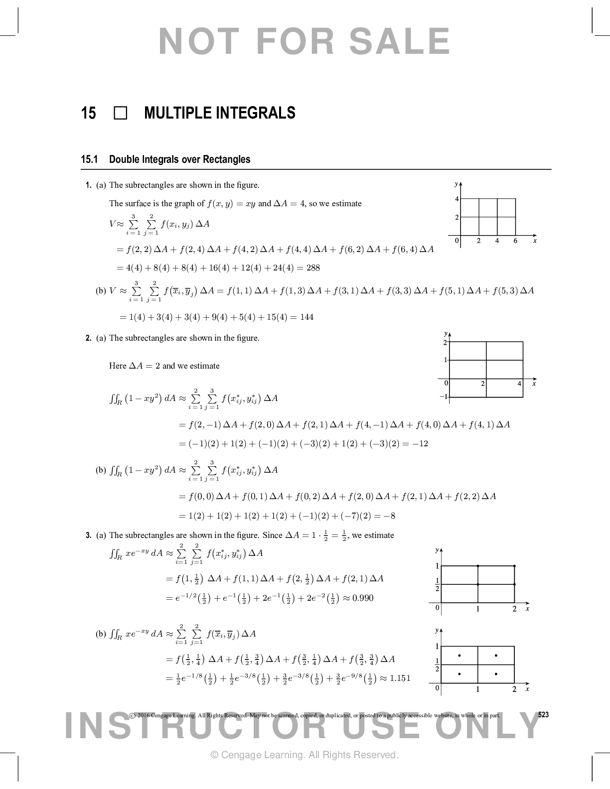
Buy this document to get the full access instantly
Instant Download Access after purchase
Add to cartInstant download
Reviews( 0 )
Document information
Connected school, study & course
About the document
Uploaded On
Jan 06, 2020
Number of pages
1
Written in

Additional information
This document has been written for:
Uploaded
Jan 06, 2020
Downloads
0
Views
61