Engineering > QUESTIONS & ANSWERS > Engineering Electromagnetics-6th-edition- by william-h-hayt-john-a-buck: All Questions Chapter 1 to (All)
Engineering Electromagnetics-6th-edition- by william-h-hayt-john-a-buck: All Questions Chapter 1 to 10 and Solutions
Document Content and Description Below
1.1. Given the vectors M = −10ax + 4ay − 8az and N = 8ax + 7ay − 2az, find: a) a unit vector in the direction of −M + 2N. Given three points, A(4, 3, 2), B(−2, 0, 5), and C(7, −2, 1): ... a) Specify the vector A extending from the origin to the point A. The vector from the origin to the point A is given as (6, 2, 4), and the unit vector directed from the origin toward point B is (2, 2, 1)/3. If points A and B are ten units apart, find the coordinates of point 1.4. given points A(8, −5, 4) and B(−2, 3, 2), find: d) the coordinates of the point on the line connecting A to B at which the line intersects the plane z 3. Note that the midpoint, (3, 1, 3), as determined from part c happens to have z coordinate of 3. This is the point we are looking for. 1.10. Use the definition of the dot product to find the interior angles at A and B of the triangle defined by the three points c) the angle between RDA and RDC : Use RDA RAD (12, 17, 14) and RDC (10, 6, 4). The angle is found through the dot product of the associated unit vectors, or The four vertices of a regular tetrahedron are located at 1.15. Three vectors extending from the origin are given as r1 = (7, 3, −2), r2 = (−2, 7, −3), and r3 = (0, 2, 3). a) a unit vector perpendicular to both r1 and r2 Evaluate D at the point where ρ = 2, φ = 0.2π, and z = 5, expressing the result in cylindrical and cartesian coordinates: At the given point, and in cylindrical coordinates, D 0.5aρ . To express this in cartesian, we use 1.20. Express in cartesian components: 1.22. A field is given in cylindrical coordinates as NOTE: The limits on the φ integration must be converted to radians (as was done here, but not shown). b) Find the total area of the enclosing surface: d) Find the length of the longest straight line that lies entirely within the volume: This will be between the points A(ρ = 3, φ = 100◦, z = 3) and B(ρ = 5, φ = 130◦, z = 4.5). Performing point transformations to cartesian coordinates, these become A(x = −0.52, y = 2.95, z = 3) and B(x = −3.21, y = 3.83, z = 4.5). Taking A and B as vectors directed from the origin, the requested length Express ar in cartesian components at Determine the cartesian components of the vector from 1.29. Express the unit vector ax in spherical components at the point: (continued) Express the unit vector ax in spherical components at the point: c) the distance from A to C on a great circle path: Note that A and C share the same r and φ coordinates; thus moving from A to C involves only a change in θ of 60◦. The requested arc length is then 2.1. Four 10nC positive charges are located in the z 0 plane at the corners of a square 8cm on a side. A fifth 10nC positive charge is located at a point 8cm distant from the other charges. Calculate the magnitude of the total force on this fifth charge for ǫ = ǫ0: Arrange the charges in the xy plane at lo√cations (4,4), (4,-4), (-4,4), and (-4,-4). Then the fifth charge will be on the z axis at location z = 4 2, which puts it at 8cm distance from the other four. By symmetry, the force on the fifth charge will be z-directed, and will be four times the z component of force produced by each of the four other charges. 2.2. A charge Q1 0.1 µC is located at the origin, while Q2 0.2 µC is at A(0.8, 0.6, 0). Find the locus of points in the z 0 plane at which the x component of the force on a third positive charge is zero. To solve this problem, the z coordinate of the third charge is immaterial, so we can place it in the xy plane at coordinates (x, y, 0). We take its magnitude to be Q3. The vector directed from the first charge to the third is R13 = xax + yay ; the vector directed from the second charge to the third is R23 = (x − 0.8)ax + (y + 0.6)ay . The force on the third charge is now 2.3. Point charges of 50nC each are located at A(1, 0, 0), B( 1, 0, 0), C(0, 1, 0), and D(0, 1, 0) in free space. Find the total force on the charge at A. The force will be: where R13 = (x − 2)ax + (y − 5)ay and R23 = (x − 6)ax + (y − 15)ay . Note, however, that all three charges must lie in a straight line, and the location of Q3 will be along the vector R12 extended past Q2. The slope of this vector is (15 5)/(6 2) 2.5. Therefore, we look for P3 at coordinates (x, 2.5x, 8). With this restriction, the force becomes: To obtain Ex 0, we require the expression in the large brackets to be zero. This expression simplifies to the following quadratic: b) What single charge at the origin would provide the identical field strength? We require where R1, R2, R3 are the vectors to P from each of the charges in their original listed order. Specifically, 2.9. A 100 nC point charge is located at A(−1, 1, 3) in free space. a) Find the locus of all points P (x, y, z) at which Ex = 500 V/m: The total field at P will be: where R1, the vector from the positive charge to point P is (−3, y, 0), and R2, the vector from the negative charge to point P , is (3, y, 0). The magnitudes of these vectors are |R1| = |R2| = 9 + y2. Substituting these into the expression for EP produces 2.11. A charge Q0 located at the origin in free space produces a field for which 2.12. The volume charge density ρv = ρ0e−|x|−|y|−|z| exists over all free space. Calculate the total charge present: This will be 8 times the integral of ρv over the first octant, or 2.13. A uniform volume charge density of 0.2 µC/m3 (note typo in book) is present throughout the spherical shell extending from r = 3 cm to r = 5 cm. If ρv = 0 elsewhere: a) find the total charge present throughout the shell: This will be b) find r1 if half the total charge is located in the region 3 cm < r < r1: If the integral over r in part a is taken to r1, we would obtain Following the same evaulation procedure as in part a, we obtain Q′ = 0.182 mC. 2.15. A spherical volume having a 2 µm radius contains a uniform volume charge density of 1015 C/m3. a) What total charge is enclosed in the spherical volume? This will be Q = (4/3)π(2 × 10−6)3 × 1015 = 3.35 × 10⁻² C. b) Now assume that a large region contains one of these little spheres at every corner of a cubical grid 3mm on a side, and that there is no charge between spheres. What is the average volume charge density throughout this large region? Each cube will contain the equivalent of one little sphere. Neglecting the little sphere volume, the average density becomes b) Find E at that point in the z = 0 plane where the direction of E is given by (1/3)ay − (2/3)az: With z = 0, the general field will be 2.19. A uniform line charge of 2 µC/m is located on the z axis. Find E in cartesian coordinates at P (1, 2, 3) if the charge extends from a) < z < : With the infinite line, we know that the field will have only a radial component in cylindrical coordinates (or x and y components in cartesian). The field from an infinite line on the z axis is generally E = [ρl /(2πǫ0ρ)]aρ . Therefore, at point P : The student is invited to verify that when evaluating the above expression over the limits −∞ < z < ∞, the z component vanishes and the x and y components become those found in part a. 2.20. Uniform line charges of 120 nC/m lie along the entire extent of the three coordinate axes. Assuming free space conditions, find E at P (−3, 2, −1): Since all line charges are infinitely-long, we can write: 2.21. Two identical uniform line charges with ρl 75 nC/m are located in free space at x 0, y 0.4 m. What force per unit length does each line charge exert on the other? The charges are parallel to the z axis and are separated by 0.8 m. Thus the field from the charge at y = −0.4 evaluated at the location of the charge at y = +0.4 will be E = [ρl /(2πǫ0(0.8))]ay . The force on a differential length of the line at the positive y location is dF dqE ρl dzE. Thus the force per unit length acting on the line at postive y arising from the charge at negative y is The force on the line at negative y is of course the same, but with −ay . 2.22. A uniform surface charge density of 5 nC/m2 is present in the region x = 0, −2 < y < 2, and all z. If ǫ = ǫ0, find E at: a) PA(3, 0, 0): We use the superposition integral: Since the integration limits are symmetric about the origin, and since the y and z components of the integrand exhibit odd parity (change sign when crossing the origin, but otherwise symmetric), these will integrate to zero, leaving only the x component. This is evident just from the symmetry of the problem. Performing the z integration first on the x component, we obtain (using tables): The student is encouraged to verify that if the y limits were −∞ to ∞, the result would be that of the infinite charged plane, or Ex = ρs /(2ǫ0). b) PB (0, 3, 0): In this case, r 3ay , and symmetry indicates that only a y component will exist. The integral becomes 2.24. Surface charge density is positioned in free space as follows: 20 nC/m2 at x 3, 30 nC/m2 at y 4, and 40 nC/m2 at z 2. Find the magnitude of E at the three points, (4, 3, 2), ( 2, 5, 1), and (0, 0, 0). Since all three sheets are infinite, the field magnitude associated with each one will be ρs /(2ǫ0), which is position-independent. For this reason, the net field magnitude will be the same everywhere, whereas the field direction will depend on which side of a given sheet one is positioned. We take the first point, for example, and find 2.25. Find E at the origin if the following charge distributions are present in free space: point charge, 12 nC at P (2, 0, 6); uniform line charge density, 3nC/m at x = −2, y = 3; uniform surface charge density, 0.2 nC/m2 at x = 2. The sum of the fields at the origin from each charge in order is: 2.26. A uniform line charge density of 5 nC/m is at y 0, z 2 m in free space, while 5 nC/m is located at y 0, z 2 m. A uniform surface charge density of 0.3 nC/m2 is at y 0.2 m, and 0.3 nC/m2 is at y 0.2 m. Find E at the origin: Since each pair consists of equal and opposite charges, the effect at the origin is to double the field produce by one of each type. Taking the sum of the fields at the origin from the surface and line charges, respectively, we find: 2.30. Given the electric field intensity E = 400yax + 400xay V/m, find: a) the equation of the streamline passing through the point A(2, 1, −2): Write: b) the equation of the surface on which |E| = 800 V/m: Have |E| = 400 x2 + y2 = 800. Thus x2 + y2 = 4, or we have a circular-cylindrical surface, centered on the z axis, and of radius 2. c) A sketch of the part a equation would yield a parabola, centered at the origin, whose axis is the positive x axis, and for which the slopes of the asymptotes are ±1. d) A sketch of the trace produced by the intersection of the surface of part b with the z 0 plane would yield a circle centered at the origin, of radius 2. 2.31. In cylindrical coordinates with E(ρ, φ) = Eρ (ρ, φ)aρ + Eφ (ρ, φ)aφ , the differential equation describ- ing the direction lines is Eρ /Eφ dρ/(ρdφ) in any constant-z plane. Derive the equation of the line passing through the point P (ρ 4,φ 10◦,z 2) in the field E 2ρ2 cos 3φaρ 2ρ2 sin 3φaφ : Using the given information, we write 3.1. An empty metal paint can is placed on a marble table, the lid is removed, and both parts are discharged (honorably) by touching them to ground. An insulating nylon thread is glued to the center of the lid, and a penny, a nickel, and a dime are glued to the thread so that they are not touching each other. The penny is given a charge of 5 nC, and the nickel and dime are discharged. The assembly is lowered into the can so that the coins hang clear of all walls, and the lid is secured. The outside of the can is again touched momentarily to ground. The device is carefully disassembled with insulating gloves and tools. a) What charges are found on each of the five metallic pieces? All coins were insulated during the entire procedure, so they will retain their original charges: Penny: 5 nC; nickel: 0; dime: 0. The penny’s charge will have induced an equal and opposite negative charge (-5 nC) on the inside wall of the can and lid. This left a charge layer of +5 nC on the outside surface which was neutralized by the ground connection. Therefore, the can retained a net charge of −5 nC after disassembly. b) If the penny had been given a charge of 5 nC, the dime a charge of 2 nC, and the nickel a charge of 1 nC, what would the final charge arrangement have been? Again, since the coins are insulated, they retain their original charges. The charge induced on the inside wall of the can and lid is equal to negative the sum of the coin charges, or 2 nC. This is the charge that the can/lid contraption retains after grounding and disassembly. 3.2. A point charge of 12 nC is located at the origin. four uniform line charges are located in the x 0 plane as follows: 80 nC/m at y 1 and 5 m, 50 nC/m at y 2 and 4 m. a) Find D at P (0, 3, 2): Note that this point lies in the center of a symmetric arrangement of line charges, whose fields will all cancel at that point. Thus D arise from the point charge alone, and will be 12 × 10−9(−3ay + 2az) 4π(3 2 ) 2 −11 ay + 4.07 × 10 −11 az C/m2 = − 61.1ay + 40.7az pC/m b) How much electric flux crosses the plane y = −3 and in what direction? The plane intercepts all flux that enters the −y half-space, or exactly half the total flux of 12 nC. The answer is thus 6 nC and in the ay direction. c) How much electric flux leaves the surface of a sphere, 4m in radius, centered at C(0, 3, 0)? This sphere encloses the point charge, so its flux of 12 nC is included. The line charge contributions are most easily found by translating the whole assembly (sphere and line charges) such that the sphere is centered at the origin, with line charges now at y 1 and 2. The flux from the line charges will equal the total line charge that lies within the sphere. The length of each of the inner two line charges (at y = ±1) will be 3.5. Let D 4xyax 2(x2 z2)ay 4yzaz C/m2 and evaluate surface integrals to find the total charge enclosed in the rectangular parallelepiped 0 < x < 2, 0 < y < 3, 0 < z < 5 m: Of the 6 surfaces to consider, only 2 will contribute to the net outward flux. Why? First consider the planes at y = 0 and 3. The y component of D will penetrate those surfaces, but will be inward at y = 0 and outward at y = 3, while having the same magnitude in both cases. These fluxes will thus cancel. At the x = 0 plane, Dx = 0 and at the z = 0 plane, Dz = 0, so there will be no flux contributions from these surfaces. This leaves the 2 remaining surfaces at x = 2 and z = 5. The net outward flux becomes: wo uniform line charges, each 20 nC/m, are located at y 1, z 1 m. Find the total flux leaving a sphere of radius 2 m if it is centered at a) A(3, 1, 0): The result will be the same if we move the sphere to the origin and the line charges to (0, 0, ±1). The length of the line charge within the sphere is given by l = 4 sin[cos−1(1/2)] = 3.46. With two line charges, symmetrically arranged, the total charge enclosed is given by Q = 2(3.46)(20 nC/m) = 139 nC b) B(3, 2, 0): In this case the result will be the same if we move the sphere to the origin and keep the charges where they were. Th√e length of the line joining the origin to the midpoint of the line charge (in the yz plane) is l1 = 2. The length of the line joining the origin to either endpoint of the line charge is then just the sp√here radius, or 2. The half-angle subtended at the origin by the line charge is then ψ = cos√−1( 2/2) = 45◦. The length of each line charge in the sphere is then l2√= 2 × 2 sin ψ = 2 2. The total charge enclosed (with two line charges) is now Q′ = 2(2 2)(20 nC/m) = 113 nC By using Gauss’s law, calculate the value of Dr on the surface r 1 mm: The gaussian surface is a spherical shell of radius 1 mm. The enclosed charge is the result of part a. We thus 3.10. Let ρs 8 µC/m2 in the region where x 0 and 4 < z < 4 m, and let ρs 0 elsewhere. Find D at P (x, 0, z), where x > 0: The sheet charge can be thought of as an assembly of infinitely-long parallel strips that lie parallel to the y axis in the yz plane, and where each is of thickness dz. The field from each strip is that of an infinite line charge, and so we can construct the field at P from a single strip as: (continued) where r xax zaz and r′ z′az We distinguish between the fixed coordinate of P , z, and the variable coordinate, z′, that determines the location of each charge strip. To find the net field at P , we sum the contributions of each strip by integrating over z′: The student is invited to verify that for very small x or for a very large sheet (allowing z′ to approach infinity), the above expression reduces to the expected form, DP ρs /2. Note also that the expression is valid for all x (positive or negative values). 3.11. In cylindrical coordinates, let ρv = 0 for ρ < 1 mm, ρv = 2 sin(2000πρ) nC/m3 for 1 mm < ρ < 1.5 mm, and ρv 0 for ρ > 1.5 mm. Find D everywhere: Since the charge varies only with radius, and is in the form of a cylinder, symmetry tells us that the flux density will be radially-directed and will be constant over a cylindrical surface of a fixed radius. Gauss’ law applied to such a surface of unit length in z gives: a) for ρ < 1 mm, D within this range. ρ = 0, since no charge is enclosed by a cylindrical surface whose radius lies b) for 1 mm < ρ < 1.5 mm, we have continued) c) for ρ > 1.5 mm, the gaussian cylinder now lies at radius ρ outside the charge distribution, so the integral that evaluates the enclosed charge now includes the entire charge distribution. To accomplish this, we change the upper limit of the integral of part b from ρ to 1.5 mm, finally obtaining: 3.12. A nonuniform volume charge density, ρv = 120r C/m3, lies within the spherical surface r = 1 m, and ρv = 0 everywhere else. a) Find Dr everywhere. For r < 1 m, we apply Gauss’ law to a spherical surface of radius r within this range to find Thus Dr (30r2) for r < 1 m. For r > 1 m, the gaussian surface lies outside the charge distribution. The set up is the same, except the upper limit of the above integral is 1 instead of r. This results in Dr = (30/r2) for r > 1 m. b) What surface charge density, ρs2, should be on the surface r = 2 such that Dr,r=2− = 2Dr,r=2+? At r = 2−, we have Dr,r=2− = 30/22 = 15/2, from part a. The flux density in the region r > 2 arising from a surface charge at r = 2 is found from Gauss’ law through The total flux density in the region r > 2 arising from the two distributions is 3.13. Spherical surfaces at r = 2, 4, and 6 m carry uniform surface charge densities of 20 nC/m2, −4 nC/m2, and ρs0, respectively. a) Find D at r 1, 3 and 5 m: Noting that the charges are spherically-symmetric, we ascertain that D will be radially-directed and will vary only with radius. Thus, we apply Gauss’ law to spherical shells in the following regions: r < 2: Here, no charge is enclosed, and so D b) Determine ρs0 such that D = 0 at r = 7 m. Since fields will decrease as 1/r2, the question could be re-phrased to ask for ρs0 such that D 0 at all points where r > 6 m. In this region, the total field will be ρv = 5 nC/m3 for 0 < ρ < 1 mm and no other charges are present: a) find Dρ for ρ < 1 mm: Applying Gauss’ law to a cylindrical surface of unit length in z, and of radius ρ < 1 mm, we find c) Evaluate Dρ at ρ = 0.8 mm, 1.6 mm, and 2.4 mm: At ρ = 0.8 mm, no charge is enclosed by a cylindrical gaussian surface of that radius, so Dρ (0.8mm) = 0. At ρ = 1.6 mm, we evaluate the part b result at ρ1 = 1.6 to obtain: 3.16. Given the electric flux density, D 2xy ax x2 ay 6z3 az C/m2: a) use Gauss’ law to evaluate the total charge enclosed in the volume 0 < x, y,z < a: We call the surfaces at x = a and x = 0 the front and back surfaces respectively, those at y = a and y = 0 the right and left surfaces, and those at z = a and z = 0 the top and bottom surfaces. To evaluate the total charge, we integrate D • n over all six surfaces and sum the results (continued) Noting that the back and bottom integrals are zero, and that the left and right integrals cancel, we evaluate the remaining two (front and top) to obtain Q = 6a5 + a4. b) use Eq. (8) to find an approximate value for the above charge. Evaluate the derivatives at P (a/2, a/2, a/2): In this application, Eq. (8) states that Q . (∇ • D )Ov. We find ∇ • D = 2x + 18z , which when evaluated at P becomes ∇• D = a + 4.5a . Thus Q = (a + 4.5a )a = 4.5a + a c) Show that the results of parts a and b agree in the limit as a → 0. In this limit, both expressions reduce to Q = a4, and so they agree. 3.17. A cube is defined by 1 < x, y,z < 1.2. If D = 2x2yax a) apply Gauss’ law to find the total flux leaving the closed surface of the cube. We call the surfaces at x 1.2 and x 1 the front and back surfaces respectively, those at y 1.2 and y 1 the right and left surfaces, and those at z 1.2 and z 1 the top and bottom surfaces. To evaluate the total charge, we integrate D n over all six surfaces and sum the results. We note that there is no z component of D, so there will be no outward flux contributions from the top and bottom surfaces. The fluxes through the remaining four are 3.18. Let a vector field by given by G 5x4y4z4 ay . Evaluate both sides of Eq. (8) for this G field and the volume defined by x 3 and 3.1, y 1 and 1.1, and z 2 and 2.1. Evaluate the partial derivatives at the center of the volume. First find The center of the cube is located at (3.05,1.05,2.05), and the volume is Ov (0.1)3 0.001. Eq. (8) then 3.19. A spherical surface of radius 3 mm is centered at P (4, 1, 5) in free space. Let D = xax C/m2. Use the results of Sec. 3.4 to estimate the net electric flux leaving the spherical surface: We use 8 . 3.20. A cube of volume a3 has its faces parallel to the cartesian coordinate surfaces. It is centered at P (3, 2, 4). Given the field D 2x3ax C/m2: a) calculate div D at P : In the present case, this will be b) evaluate the fraction in the rightmost side of Eq. (13) for a = 1 m, 0.1 m, and 1 mm: With the field having only an x component, flux will pentrate only the two surfaces at x = 3 ± a/2, each of which has surface area a2. The cube volume is Ov = a3. The equation reads: a) Find div D: Using the divergence formula for cylindrical coordinates (see problem 3.21), we find ∇• D = 12 sin φ. b) Find the volume charge density at P (2.6, 38◦, −6.1): Since ρv =∇ • D, we evaluate the result of part a at this point to find ρvP = 12 sin 38◦ = 7.39 C/m3. c) How much charge is located inside the region defined by 0 A point charge Q lies at the origin. Show that div D is zero everywhere except at the origin. For a point charge at the origin we know that D Q/(4πr2) ar . Using the formula for divergence in spherical coordinates (see problem 3.21 solution), we find in this case that The above is true provided r > 0. When r 0, we have a singularity in D, so its divergence is not defined. b) Replace the point charge with a uniform volume charge density ρv0 for 0 < r < a. Relate ρv0 to Q and a so that the total charge is the same. Find div D everywhere: To achieve the same net charge, we require that (4/3)πa3ρv0 Q, so ρv0 3Q/(4πa3) C/m3. Gauss’ law tells us that inside the charged sphere . How much electric flux leaves the closed surface 3 < ρ < 4, 0 < φ < 2π, 2.5 < z < 2.5? We note that D has only a radial component, and so flux would leave only through the cylinder sides. Also, D does not vary with φ or z, so the flux is found by a simple product of the side area and the flux density. We further note that D 0 at ρ 3, so only the outer side (at ρ 4) will contribute. We use the result of part b, and write the flux as ) How much charge is contained within the volume used in part c? By Gauss’ law, this will be the same as the net outward flux through that volume, or again, 200π C. 3.25. Within the spherical shell, 3 < r < 4 m, the electric flux density is given as which we evaluate at r = 4 to find ρv (r = 4) = 17.50 C/m3. b) What is the electric flux density at r = 4? Substitute r = 4 into the given expression to find D(4) = 5 ar C/m2 c) How much electric flux leaves the sphere r = 4? Using the result of part b, this will be 8 = 4π(4)2(5) = 320π C d) How much charge is contained within the sphere, r = 4? From Gauss’ law, this will be the same as the outward flux, or again, Q = 320π C. 3.26. Given the field 26d. the total electric flux leaving the surface r 2 Since the total enclosed charge is zero (from part b), the net outward flux is also zero, from Gauss’ law. 3.27. Let D 5.00r2ar mC/m2 for r 0.08 m and D 0.205 ar /r2 µC/m2 for r 0.08 m (note error in problem statement). a) Find ρv for r = 0.06 m: This radius lies within the first region, and so b) Find ρv for r 0.1 m: This is in the region where the second field expression is valid. The 1/r2 dependence of this field yields a zero divergence (shown in Problem 3.23), and so the volume charge density is zero at 0.1 m. c) What surface charge density could be located at r 0.08 m to cause D 0 for r > 0.08 m? The total surface charge should be equal and opposite to the total volume charge. The latter is 3.28. The electric flux density is given as D = 20ρ3 aρ C/m2 for ρ < 100 µm, and k aρ /ρ for ρ > 100 µm. a) Find k so that D is continuous at ρ = 100 µm: We require b) Find and sketch ρv as a function of ρ: In cylindrical coordinates, with only a radial component of D, we use . Evaluate the surface integral side for the corresponding closed surface: We call the surfaces at x 3 and x 2 the front and back surfaces respectively, those at y 3 and y 2 the right and left surfaces, and those at z 3 and z 2 the top and bottom surfaces. To evaluate the surface integral side, we integrate D n over all six surfaces and sum the results. Note that since the x component of D does not vary with x, the outward fluxes from the front and back surfaces will cancel each other. The same is true for the left and right surfaces, since Dy does not vary with y. This leaves only the top and bottom surfaces, where the fluxes are: 3.30. If D 15ρ2 sin 2φ aρ 10ρ2 cos 2φ aφ C/m2, evaluate both sides of the divergence theorem for the region 1 < ρ < 2 m, 1 < φ < 2 rad, 1 < z < 2 m: Taking the surface integral side first, the six sides over which the flux must be evaluated are only four, since there is no z component of D. We are left with the sides at φ 1 and φ 2 rad (left and right sides, respectively), and those at ρ 1 and ρ 2 (back and front sides). We evaluate use two different methods to find the total charge within the region 1 < r < 2 m, 1 < θ < 2 rad, 1 < φ < 2 rad: We use the divergence theorem and first evaluate the surface integral side. We are evaluating the net outward flux through a curvilinear “cube”, whose boundaries are defined by the specified ranges. The flux contributions will be only through the surfaces of constant θ , however, since D has only a θ component. On a constant-theta surface, the differential area is da r sin θdrdφ, where θ is fixed at the surface location. Our flux integral becomes 4.1. The value of E at P (ρ 2, φ 40◦, z 3) is given as E 100aρ 200aφ 300az V/m. Determine the incremental work required to move a 20 µC charge a distance of 6 µm: a) in the direction of aρ : The incremental work is given by dW = −q E • dL, where in this case, dL = dρ aρ = 6 × 10⁻⁶ aρ . Thus 4.2. Let E 400ax 300ay 500az in the neighborhood of point P (6, 2, 3). Find the incremental work done in moving a 4-C charge a distance of 1 mm in the direction specified by: a) ax + ay + az: We write b) Q(2, 1, 4) toward P (1, 2, 3): A little thought is in order here: Note that the field has only a ra√dial component and does not depend on φ or z. Note also that P and Q are at the same radius ( 5) from the z axis, but have different φ and z coordinates. We could just as well position the two points at the same z location and the problem would not change. If this were so, then moving along a st√raight line between P and Q would thus involve moving along a chord of a circle whose radius is 5. Halfway along this line is a point of symmetry in the field (make a sketch to see this). This means that when starting from either point, the initial force will be the same. Thus the answer is dW 3.1 µJ as in part a. This is also found by going through the same procedure as in part a, but with the direction (roles of P and Q) reversed. 4.8. A point charge Q1 is located at the origin in free space. Find the work done in carrying a charge Q2 from: (a) B(rB , θB , φB ) to C(rA, θB , φB ) with θ and φ held constant; (b) C(rA, θB , φB ) to D(rA, θA, φB ) with r and φ held constant; (c) D(rA, θA, φB ) to A(rA, θA, φA) with r and θ held constant: The general expression for the work done in this instance is The answers to parts b and c (involving paths over which r is held constant) are both 0. 4.9. A uniform surface charge density of 20 nC/m2 is present on the spherical surface r 0.6 cm in free space. a) Find the absolute potential at P (r 1 cm, θ 25◦, φ 50◦): Since the charge density is uniform and is spherically-symmetric, the angular coordinates do not matter. The potential function for r > 0.6 cm will be that of a point charge of Q = 4πa2ρs , or 4.10. Given a surface charge density of 8 nC/m2 on the plane x = 2, a line charge density of 30 nC/m on the line x 1, y 2, and a 1-µC point charge at P ( 1, 1, 2), find VAB for points A(3, 4, 0) and B(4, 0, 1): We need to find a potential function for the combined charges. That for the point charge we know to be Potential functions for the sheet and line charges can be found by taking indefinite integrals of the electric fields for those distributions. For the line charge, we have The terms in this expression are not referenced to a common origin, since the charges are at different positions. The parameters r, ρ, and x are scalar distances from the charges, and will be treated as such here. For point A we have r 4.11. Let a uniform surface charge density of 5 nC/m2 be present at the z 0 plane, a uniform line charge density of 8 nC/m be located at x 0, z 4, and a point charge of 2 µC be present at P (2, 0, 0). If V 0 at M(0, 0, 5), find V at N(1, 2, 3): We need to find a potential function for the combined charges which is zero at M. That for the point charge we know to be Potential functions for the sheet and line charges can be found by taking indefinite integrals of the electric fields for those distributions. For the line charge, we have The total potential function will be the sum of the three. Combining the integration constants, we obtain continued) The terms in this expression are not referenced to a common origin, since the charges are at different positions. The parameters r, ρ, and z are scalar distances from the charges, and will be treate√d as such he√re. To evaluate the constant, C, we first look at point M, where VT = 0. At M, r = 22 + 52 = 29, ρ = 1, and z = 5. We thus have 4.12. Three point charges, 0.4 µC each, are located at (0, 0, 1), (0, 0, 0), and (0, 0, 1), in free space. a) Find an expression for the absolute potential as a function of z along the line x 0, y 1: From a point located at position z along the given line, the distances to the three charges are R1 = ,(z − 1)2 + 1, R2 = √z2 + 1, and R3 = ,(z + 1)2 + 1. The total potential will be 4.13. Three identical point charges of 4 pC each are located at the corners of an equilateral triangle 0.5 mm on a side in free space. How much work must be done to move one charge to a point equidistant from the other two and on the line joining them? This will be the magnitude of the charge times the potential difference between the finishing and starting positions, or 4.16. Uniform surface charge densities of 6, 4, and 2 nC/m2 are present at r 2, 4, and 6 cm, respectively, in free space. a) Assume V 0 at infinity, and find V(r). We keep in mind the definition of absolute potential as the work done in moving a unit positive charge from infinity to location r. At radii outside all three spheres, the potential will be the same as that of a point charge at the origin, whose charge is the sum of the three sphere charges: 4.20. Fig. 4.11 shows three separate charge distributions in the z 0 plane in free space. a) find the total charge for each distribution: Line charge along the y axis: c) the total charge lying within the surface r 0.6: The easiest way is to use Gauss’ law, and integrate the flux density over the spherical surface r 0.6. Since the field is constant at constant radius, we obtain the product: the total charge lying within the closed surface ρ = .6, 0 < z < 1: The easiest way to do this calculation is to evaluate Dρ at ρ = .6 (noting that it is constant), and then multiply by the cylinder area: Using part a, we have Dρ ..64.24. Given the potential field V = 80r2 cos θ and a point P (2.5,θ = 30◦,φ = 60◦) in free space, find at P : a) V : Substitute the coordinates into the function and find VP = 80(2.5)2 cos(30) = 433 V. b) E: 4.26. A dipole having Qd/(4πǫ0) = 100 V • m2 is located at the origin in free space and aligned so that its moment is in the az direction. a) Sketch |V(r = 1,θ,φ = 0)| versus θ on polar graph paper (homemade if you wish). b) Sketch |E(r = 1,θ,φ = 0)| versus θ on polar graph paper: Taking the magnitude of the above, we find |EP |= 25.2 V/m. c) Now treat the two√charges as a dipole at the origin and find V at P : In spherical coordinates, P is located at r we have 4.28. A dipole located at the origin in free space has a moment p2 × 10−9 az C • m. At what points on the line y = z, x = 0 is: The y and z values are thus y = z = ±23.3/√2 = ±16.5m b) Er 1 mV/m? From the above field expression, the radial component magnitude is twice that of the theta component. Using the same development, we then find 4.29. A dipole having a moment p 3ax 5ay 10az nC m is located at Q(1, 2, 4) in free space. Find V at P (2, 3, 4): We use the general expression for the potential in the far field: 4.30. A dipole, having a moment p 2az nC m is located at the origin in free space. Give the magnitude of E and its direction aE in cartesian components at r 100 m, φ 90◦, and θ : a) 0◦; b) 30◦; c) 90◦. Begin with Show that the surface θ = 0.6π is an equipotential surface: This will be the surface of a cone, centered at the origin, along which E, in the ar direction, will exist. Therefore, the given surface cannot be an equipotential (the problem was ill-conceived). Only a surface of constant r could be an equipotential in this field. c) Find VAB 4.33. A copper sphere of radius 4 cm carries a uniformly-distributed total charge of 5 µC in free space. a) Use Gauss’ law to find D external to the sphere: with a spherical Gaussian surface at radius r, D will be the total charge divided by the area of this sphere, and will be ar -directed. Thus 4.34. Given the potential field in free space, V 80φ V (note that aphi should not be present), find: a) the energy stored in the region 2 < ρ < 4 cm, 0 < φ < 0.2π, 0 < z < 1 m: First we find 4.34c. the maximum value of the energy density in the specified region: The energy density is This will maximize at the lowest value of ρ in the specified range, which is ρ = 2 cm. So 4.35. Four 0.8 nC point charges are located in free space at the corners of a square 4 cm on a side. a) Find the total potential energy stored: This will be given by where Vn in this case is the potential at the location of any one of the point charges that arises from the other three. This will be (for charge 1) Taking the summation produces a factor of 4, since the situation is the same at all four points. Consequently, b) A fifth 0.8 µC charge is installed at the center of the square. Again find the total stored energy: This will be the energy found in part a plus the amount of work done in moving the fifth charge into position from infinity. The latter is just the potential at the square center arising from the original four charges, times the new charge value, or 5.1. Given the current density J = −104[sin(2x)e−2y ax + cos(2x)e−2y ay ] kA/m2: a) Find the total current crossing the plane y 1 in the ay direction in the region 0 < x < 1, 0 < z < 2: This is found through b) Find the total current leaving the region 0 < x, x < 1, 2 < z < 3 by integrating J dS over the surface of the cube: Note first that current through the top and bottom surfaces will not exist, since J has no z component. Also note that there will be no current through the x = 0 plane, since Jx = 0 there. Current will pass through the three remaining surfaces, and will be found through c) Repeat part b, but use the divergence theorem: We find the net outward current through the surface of the cube by integrating the divergence of J over the cube volume. We have Make the assumption that the electrons are emitted continuously as a beam with a 0.25 mm radius and a total current of 60 µA. Find J(z) and ρ(z): (negative since we have electrons flowing in the positive z direction) Next we use J(z) = ρv (z)v(z), d) Show that the divergence theorem is satisfied for J and the surface specified in part b. In part c, the net outward flux was found to be zero, and in part b, the divergence of J was found to be zero (as will be its volume integral). Therefore, the divergence theorem is satisfied. 5.7. Assuming that there is no transformation of mass to energy or vice-versa, it is possible to write a continuity equation for mass. a) If we use the continuity equation for charge as our model, what quantities correspond to J and ρv ? These would be, respectively, mass flux density in (kg/m2 − s) and mass density in (kg/m3). b) Given a cube 1 cm on a side, experimental data show that the rates at which mass is leaving each of the six faces are 10.25, -9.85, 1.75, -2.00, -4.05, and 4.45 mg/s. If we assume that the cube is an incremental volume element, determine an approximate value for the time rate of change of density at its center. We may write the continuity equation for mass as follows, also invoking the divergence theorem: 5.8. The continuity equation for mass equates the divergence of the mass rate of flow (mass per second per square meter) to the negative of the density (mass per cubic meter). After setting up a cartesian coordinate system inside a star, Captain Kirk and his intrepid crew make measurements over the faces of a cube centered at the origin with edges 40 km long and parallel to the coordinate axes. They find the mass rate of flow of material outward across the six faces to be -1112, 1183, 201, -196, 1989, and -1920 kg/m2 s. a) Estimate the divergence of the mass rate of flow at the origin: We make the estimate using the definition of divergence, but without taking the limit as the volume shrinks to zero: Using data tabulated in Appendix C, calculate the required diameter for a 2-m long nichrome wire that will dissipate an average power of 450 W when 120 V rms at 60 Hz is applied to it: The required resistance will be 5.10. A steel wire has a radius of 2 mm and a conductivity of 2 106 S/m. The steel wire has an aluminum (σ 3.8 107 S/m) coating of 2 mm thickness. Let the total current carried by this hybrid conductor be 80 A dc. Find: a) Jst . We begin with the fact that electric field must be the same in the aluminum and steel regions. This comes from the requirement that E tangent to the boundary between two media must be continuous, and from the fact that when integrating E over the wire length, the applied voltage value must be obtained, regardless of the medium within which this integral is evaluated. We can therefore write The net current is now expressed as the sum of the currents in each region, written as the sum of the products of the current densities in each region times the appropriate cross-sectional area: 5.11. Two perfectly-conducting cylindrical surfaces are located at ρ 3 and ρ 5 cm. The total current passing radially outward through the medium between the cylinders is 3 A dc. Assume the cylinders are both of length l. a) Find the voltage and resistance between the cylinders, and E in the region between the cylinders, if a conducting material having σ 0.05 S/m is present for 3 < ρ < 5 cm: Given the current, and knowing that it is radially-directed, we find the current density by dividing it by the area of a cylinder of radius ρ and length l: 5.12. The spherical surfaces r 3 and r 5 cm are perfectly conducting, and the total current passing radially outward through the medium between the surfaces is 3 A dc. a) Find the voltage and resistance between the spheres, and E in the region between them, if a conducting material having σ 0.05 S/m is present for 3 < r < 5 cm. We first find J as a function of radius by dividing the current by the area of a sphere of radius r: 5.13. A hollow cylindrical tube with a rectangular cross-section has external dimensions of 0.5 in by 1 in and a wall thickness of 0.05 in. Assume that the material is brass, for which σ 1.5 107 S/m. A current of 200 A dc is flowing down the tube. a) What voltage drop is present across a 1m length of the tube? Converting all measurements to meters, the tube resistance over a 1 m length will be: The voltage drop is now V = I R1 = 200(7.38 × 10−4 = 0.147 V. b) Find the voltage drop if the interior of the tube is filled with a conducting material for which σ = 1.5 × 10⁵ S/m: The resistance of the filling will be: b) Find a unit vector directed outward to the surface, assuming the origin is inside the surface: Such a unit normal can be construced from the result of part c: b) Show that the z = 0 surface is an equipotential surface: There are two reasons for this: 1) E at z = 0 is everywhere z-directed, and so moving a charge around on the surface involves doing no work; 2) When evaluating the given potential function at z = 0, the result is 0 for all x and y. c) Assume that the z = 0 surface is a conductor and find the total charge on that portion of the conductor defined by 0 < x < 2, −3 < y < 0: We have where the integration “constants” are functions of all variables other than the integration variable. The general procedure is to adjust the functions, f , such that the result for V is the same in all three integrations. In this case we see that f (x, y) = f (x, z) = f (y, z) = 0 accomplishes this, and the potential function is V = −3xy2z3 as given. d) Determine VPQ, given Q(1, 1, 1): Using the potential function of part c, we have a) Determine the equations of the equipotential surfaces on which V 0 and 60 V: Setting the given potential function equal to 0 and 60 and simplifying results in: b) Assume these are conducting surfaces and find the surface charge density at that point on the V 60 V surface where x 2 and z 1. It is known that 0 V 60 V is the field-containing region: First, on the 60 V surface, we have 5.24. The mobilities for intrinsic silicon at a certain temperature are µe 0.14 m2/V s and µh 0.035 m2/V s. The concentration of both holes and electrons is 2.2 1016 m−3. Determine both the conductivity and the resistivity of this silicon 5.25. Electron and hole concentrations increase with temperature. For pure silicon, suitable expressions are ρh ρe 6200T 1.5e−7000/T C/m3. The functional dependence of the mobilities on temperature is given by µh 2.3 105T −2.7 m2/V s and µe 2.1 105T −2.5 m2/V s, where the temperature, T , is in degrees Kelvin. The conductivity will thus be 5.26. A little donor impurity, such as arsenic, is added to pure silicon so that the electron concentration is 2 1017 conduction electrons per cubic meter while the number of holes per cubic meter is only 1.1 1015. If µe 0.15 m2/V s for this sample, and µh 0.045 m2/V s, determine the conductivity and resistivity 5.27. Atomic hydrogen contains 5.5 1025 atoms/m3 at a certain temperature and pressure. When an electric field of 4 kV/m is applied, each dipole formed by the electron and positive nucleus has an effective length of 7.1 10−19 m. a) Find P: With all identical dipoles, we have This normal will point in the direction of increasing f , which will be away from the origin, or into region 2 (you can visualize a portion of the surface as a tri√angle whose vertices are on the three coordinate axes at x = 5, y = −5, and z = 2.5). So EN 1 = (1/ 6)[100 − 200 − 100] = −81.7 V/m. Since the magnitude is negative, the normal component points into region 1 from the surface. Then 5.34. Let the spherical surfaces r = 4 cm and r = 9 cm be separated by two perfect dielectric shells, ǫR1 = 2 for 4 < r < 6 cm and ǫR2 = 5 for 6 < r < 9 cm. If E1 = (2000/r2)ar V/m, find: a) E2: Since E is normal to the interface between ǫR1 and ǫR2, D will be continuous across the boundary, and so 5.37. Capacitors tend to be more expensive as their capacitance and maximum voltage, Vmax , increase. The voltage Vmax is limited by the field strength at which the dielectric breaks down, EBD . Which of these dielectrics will give the largest CVmax product for equal plate areas: (a) air: ǫR = 1, EBD = 3 MV/m; (b) barium titanate: ǫR = 1200, EBD = 3 MV/m; (c) silicon dioxide: ǫR = 3.78, EBD = 16 MV/m; (d) polyethylene: ǫR = 2.26, EBD = 4.7 MV/m? Note that Vmax = EBDd, where d is the plate separation. Also, C = ǫR ǫ0A/d, and so Vmax C = ǫR ǫ0AEBD , where A is the plate area. The maximum CVmax product is found through the maximum ǫR EBD product. Trying this with the given materials yields the winner, which is barium titanate. 5.39. A parallel plate capacitor is filled with a nonuniform dielectric characterized by ǫR = 2 + 2 × 106x2, where x is the distance from one plate. If S = 0.02 m2, and d = 1 mm, find C: Start by assuming charge density ρs on the top plate. D will, as usual, be x-directed, originating at the top plate and terminating on the bottom plate. The key here is that D will be constant over the distance between plates. This can be understood by considering the x-varying dielectric as constructed of many thin layers, each having constant permittivity. The permittivity changes from layer to layer to approximate the given function of x. The approximation becomes exact as the layer thicknesses approach zero. We know that D, which is normal to the layers, will be continuous across each boundary, and so D is constant over the plate separation distance, and will be given in magnitude by ρs . The electric field magnitude is now 0a. The width of the region containing ǫR1 in Fig. 5.19 is 1.2 m. Find ǫR1 if ǫR2 = 2.5 and the total capacitance is 60 nF: The plate areas associated with each capacitor are A1 = 1.2(2) = 2.4 m2 and A2 = 0.8(2) = 1.6 m2. Having parallel capacitors, the capacitances will add, so b) Find the width of each region (containing ǫR1 and ǫR2) if Ctotal = 80 nF, ǫR2 = 3ǫR1, and C1 = 2C2: Let w1 be the width of region 1. The above conditions enable us to write 5.41. Let ǫR1 = 2.5 for 0 < y < 1 mm, ǫR2 = 4 for 1 < y < 3 mm, and ǫR3 for 3 < y < 5 mm. Conducting surfaces are present at y = 0 and y = 5 mm. Calculate the capacitance per square meter of surface area if: a) ǫR3 is that of air; b) ǫR3 ǫR1; c) ǫR3 ǫR2; d) ǫR3 is silver: The combination will be three capacitors in series, for which (continued) The charge on a unit length of the inner conductor is Q 2π(0.8)(1)ρs . The capacitance is now Q 2π(0.8)(1)ρs C = = = 4πǫ = 111 pF/m V0 0.4ρs /ǫ0 0 Note that throughout this problem, I left all dimensions in cm, knowing that all cm units would cancel, leaving the units of capacitance to be those used for ǫ0. 5.43. Two coaxial conducting cylinders of radius 2 cm and 4 cm have a length of 1m. The region between the cylinders contains a layer of dielectric from ρ = c to ρ = d with ǫR = 4. Find the capacitance if a) c = 2 cm, d = 3 cm: This is two capacitors in series, and so 5.44. Conducting cylinders lie at ρ = 3 and ρ = 12 mm; both extend from z = 0 to z = 1 m. Perfect dielectrics occupy the interior region: ǫR = 1 for 3 < ρ < 6 mm, ǫR = 4 for 6 < ρ < 9 mm, and ǫR 8 for 9 < ρ < 12 mm. a) Calculate C: First we know that D (3ρs /ρ)aρ C/m2, with ρ expressed in mm. Then, with ρ in mm, b) A portion of the dielectric is now removed so that ǫR 1.0, 0 < φ < π/2, and ǫR 8, π/2 < φ < 2π. Again, find C: We recognize here that removing that portion leaves us with two capacitors in parallel (whose C’s will add). We use the fact that with the dielectric completely removed, the capacitance would be C(ǫR 1) 53.3/8 6.67 pF. With one-fourth the dielectric removed, the total capacitance will be 5.49. A 2 cm diameter conductor is suspended in air with its axis 5 cm from a conducting plane. Let the potential of the cylinder be 100 V and that of the plane be 0 V. Find the surface charge density on the: a) cylinder at a point nearest the plane: The cylinder will image across the plane, producing an equivalent two-cylinder problem, with the second one at location 5 cm below the plane. We will 6.1 Construct a curvilinear square map for a coaxial capacitor of 3-cm inner radius and 8-cm outer radius. These dimensions are suitable for the drawing. a) Use your sketch to calculate the capacitance per meter length, assuming ǫR 1: The sketch is shown below. Note that only a 9◦ sector was drawn, since this would then be duplicated 40 times around the circumference to complete the drawing. The capacitance is thus 6.2 Construct a curvilinear-square map of the potential field about two parallel circular cylinders, each of 2.5 cm radius, separated by a center-to-center distance of 13cm. These dimensions are suitable for the actual sketch if symmetry is considered. As a check, compute the capacitance per meter both from your sketch and from the exact formula. Assume ǫR = 1. Symmetry allows us to plot the field lines and equipotentials over just the first quadrant, as is done in the sketch below (shown to one-half scale). The capacitance is found from the formula C = (NQ/NV )ǫ0, where NQ is twice the number of squares around the perimeter of the half-circle and NV is twice the number of squares between the half-circle and the left vertical plane. The result is 6.3. Construct a curvilinear square map of the potential field between two parallel circular cylinders, one of 4-cm radius inside one of 8-cm radius. The two axes are displaced by 2.5 cm. These dimensions are suitable for the drawing. As a check on the accuracy, compute the capacitance per meter from the sketch and from the exact expression: The drawing is shown below. Use of the exact expression above yields a capacitance value of C = 11.5ǫ0 F/m. Use of the drawing produces: 6.4. A solid conducting cylinder of 4-cm radius is centered within a rectangular conducting cylinder with a 12-cm by 20-cm cross-section. a) Make a full-size sketch of one quadrant of this configuration and construct a curvilinear-square map for its interior: The result below could still be improved a little, but is nevertheless sufficient for a reasonable capacitance estimate. Note that the five-sided region in the upper right corner has been partially subdivided (dashed line) in anticipation of how it would look when the next-level subdivision is done (doubling the number of field lines and equipotentials). b) Assume ǫ ǫ0 and estimate C per meter length: In this case NQ is the number of squares around the full perimeter of the circular conductor, or four times the number of squares shown in the drawing. NV is the number of squares between the circle and the rectangle, or 5. The capacitance is estimated to be 6.5. The inner conductor of the transmission line shown in Fig. 6.12 has a square cross-section 2a 2a, while the outer square is 5a 5a. The axes are displaced as shown. (a) Construct a good-sized drawing of the transmission line, say with a 2.5 cm, and then prepare a curvilinear-square plot of the electrostatic field between the conductors. (b) Use the map to calculate the capacitance per meter length if ǫ = 1.6ǫ0. (c) How would your result to part b change if a = 0.6 cm? a) The plot is shown below. Some improvement is possible, depending on how much time one wishes to spend. 6.6. Let the inner conductor of the transmission line shown in Fig. 6.12 be at a potential of 100V, while the outer is at zero potential. Construct a grid, 0.5a on a side, and use iteration to find V at a point that is a units above the upper right corner of the inner conductor. Work to the nearest volt: The drawing is shown below, and we identify the requested voltage as 38 V. 6.7. Use the iteration method to estimate the potentials at points x and y in the triangular trough of Fig. 6.13. Work only to the nearest volt: The result is shown below. The mirror image of the values shown occur at the points on the other side of the line of symmetry (dashed line). Note that Vx = 78 V and Vy = 26 V. 6.8. Use iteration methods to estimate the potential at point x in the trough shown in Fig. 6.14. Working to the nearest volt is sufficient. The result is shown below, where we identify the voltage at x to be 40 V. Note that the potentials in the gaps are 50 V. 6.9. Using the grid indicated in Fig. 6.15, work to the nearest volt to estimate the potential at point A: The voltages at the grid points are shown below, where VA is found to be 19 V. Half the figure is drawn since mirror images of all values occur across the line of symmetry (dashed line). 6.10. Conductors having boundaries that are curved or skewed usually do not permit every grid point to coincide with the actual boundary. Figure 6.16a illustrates the situation where the potential at V0 is to be estimated in terms of V1, V2, V3, and V4, and the unequal distances h1, h2, h3, and h4. a) Show that 6.11. Consider the configuration of conductors and potentials shown in Fig. 6.17. Using the method described in Problem 10, write an expression for Vx (not V0): The result is shown below, where Vx = 70 V. a) After estimating potentials for the configuation of Fig. 6.18, use the iteration method with a square grid 1 cm on a side to find better estimates at the seven grid points. Work to the nearest volt: Construct a 0.5 cm grid, establish new rough estimates, and then use the iteration method on the 0.5 cm grid. Again, work to the nearest volt: The result is shown below, with values for the original grid points underlined: Use the computer to obtain values for a 0.25 cm grid. Work to the nearest 0.1 V: Values for the left half of the configuration are shown in the table below. Values along the vertical line of symmetry are included, and the original grid values are underlined. 6.13. Perfectly-conducting concentric spheres have radii of 2 and 6 cm. The region 2 < r < 3 cm is filled with a solid conducting material for which σ = 100 S/m, while the portion for which 3 < r < 6 cm has σ = 25 S/m. The inner sphere is held at 1 V while the outer is at V = 0. a. Find E and J everywhere: From symmetry, E and J will be radially-directed, and we note the fact that the current, I , must be constant at any cross-section; i.e., through any spherical surface at radius r between the spheres. Thus we require that in both regions, 6.14. The cross-section of the transmission line shown in Fig. 6.12 is drawn on a sheet of conducting paper with metallic paint. The sheet resistance is 2000 K/sq and the dimension a is 2 cm. a) Assuming a result for Prob. 6b of 110 pF/m, what total resistance would be measured between the metallic conductors drawn on the conducting paper? We assume a paper thickness of t m, so that the capacitance is C 110t pF, and the surface resistance is Rs 1/(σ t ) 2000 K/sq. We now use 6.15. two concentric annular rings are painted on a sheet of conducting paper with a highly conducting metal paint. The four radii are 1, 1.2, 3.5, and 3.7 cm. Connections made to the two rings show a resistance of 215 ohms between them. a) What is Rs for the conducting paper? Using the two radii (1.2 and 3.5 cm) at which the rings are at their closest separation, we first evaluate the capacitance: b) If the conductivity of the material used as the surface of the paper is 2 S/m, what is the thickness of the coating? We use 6.16. The square washer shown in Fig. 6.19 is 2.4 mm thick and has outer dimensions of 2.5 2.5 cm and inner dimensions of 1.25 1.25 cm. The inside and outside surfaces are perfectly-conducting. If the material has a conductivity of 6 S/m, estimate the resistance offered between the inner and outer surfaces (shown shaded in Fig. 6.19). A few curvilinear squares are suggested: First we find the surface resistance, Rs = 1/(σ t ) = 1/(6 × 2.4 × 10−3) = 69.4 K/sq. Having found this, we can construct the total resistance by using the fundamental square as a building block. Specifically, R = Rs (Nl /Nw) where Nl is the number of squares between the inner and outer surfaces and Nw is the number of squares around the perimeter of the washer. These numbers are found from the curvilinear square plot shown below, which covers one-eighth the washer. The resistance is thus R . 69.4[4/(8 × 5)] . 6.9 K. 6.17. A two-wire transmission line consists of two parallel perfectly-conducting cylinders, each having a radius of 0.2 mm, separated by center-to-center distance of 2 mm. The medium surrounding the wires has ǫR 3 and σ 1.5 mS/m. A 100-V battery is connected between the wires. Calculate: a) the magnitude of the charge per meter length on each wire: Use 6.18. A coaxial transmission line is modelled by the use of a rubber sheet having horizontal dimensions that are 100 times those of the actual line. Let the radial coordinate of the model be ρm. For the line itself, let the radial dimension be designated by ρ as usual; also, let a 0.6 mm and b 4.8 mm. The model is 8 cm in height at the inner conductor and zero at the outer. If the potential of the inner conductor is 100 V: a) Find the expression for V (ρ): Assuming charge density ρs on the inner conductor, we use Gauss’ Law to find 2πρD 2πaρs , from which E D/ǫ aρs /(ǫρ) in the radial direction. The potential difference between inner and outer conductors is Now, as a function of radius, and assuming zero potential on the outer conductor, the potential function will be: b) Write the model height as a function of ρm (not ρ): We use the part a result, since the gravitational function must be the same as that for the electric potential. We replace V0 by the maximum height, and multiply all dimensions by 100 to obtain: Conciliate your results with the uniqueness theorem: Uniqueness specifies that there is only one potential that will satisfy all the given boundary conditions. While both potentials have the same value at r = 4, they do not as r → ∞. So they apply to different situations. 7.10. Conducting planes at z = 2cm and z = 8cm are held at potentials of −3V and 9V, respectively. The region between the plates is filled with a perfect dielectric with ǫ 5ǫ0. Find and sketch: a) V (z): We begin with the general solution of the one-dimensional Laplace equation in rectangular coordinates: V (z) = Az + B. Applying the boundary conditions, we write −3 = A(2) + B and 9 = A(8) + B. Subtracting the former equation from the latter, we find 12 = 6A or A = 2 V/cm. Using this we find B = −7 V. Finally, V (z) = 2z − 7V (z in cm) or V (z) = 200z − 7V (z in m). 7.11. The conducting planes 2x + 3y = 12 and 2x + 3y = 18 are at potentials of 100 V and 0, respectively. Let ǫ = ǫ0 and find: a) V at P (5, 2, 6): The planes are parallel, and so we expect variation in potential in the direction normal to them. Using the two boundary condtions, our general potential function can be written: 7.12. Conducting cylinders at ρ 2 cm and ρ 8 cm in free space are held at potentials of 60mV and -30mV, respectively. a) Find V (ρ): Working in volts and meters, we write the general one-dimensional solution to the Laplace equation in cylindrical coordinates, assuming radial variation: V (ρ) = A ln(ρ) + B. Applying the given boundary conditions, this becomes V (2cm) = .060 = A ln(.02) + B and V (8cm) = −.030 = A ln(.08) + B. Subtracting the former equation from the latter, we find −.090 = A ln(.08/.02) = A ln 4 ⇒ A = −.0649. B is then found through either equation 7.13. Coaxial conducting cylinders are located at ρ = 0.5 cm and ρ = 1.2 cm. The region between the cylinders is filled with a homogeneous perfect dielectric. If the inner cylinder is at 100V and the outer at 0V, find: a) the location of the 20V equipotential surface: From Eq. (16) we have 7.14. Two semi-infinite planes are located at φ = −α and φ = α, where α < π/2. A narrow insulating strip separates them along the z axis. The potential at φ = −α is V0, while V = 0 at φ = α. a) Find V (φ) in terms of α and V0: We use the one-dimensional solution form for Laplace’s equation assuming variation along φ: V (φ) = Aφ + B. The boundary conditions are then substituted: V0 = −Aα + B and 0 = Aα + B. Subtract the latter equation from the former to obtain: V0 = −2Aα ⇒ A = −V0/(2α). Then 0 = −V0/(2α)α + B ⇒ B = V0/2. Finally V (φ) = V0 .1 − φ Σ V 7.15. The two conducting planes illustrated in Fig. 7.8 are defined by 0.001 < ρ < 0.120 m, 0 < z < 0.1 m, φ 0.179 and 0.188 rad. The medium surrounding the planes is air. For region 1, 0.179 < φ < 0.188, neglect fringing and find: a) V (φ): The general solution to Laplace’s equation will be V = C1φ + C2, and so ) Solve Laplace’s equation for the potential field in the homogeneous region between two concentric conducting spheres with radii a and b, b > a, if V 0 at r b and V V0 at r a. With radial variation only, we have Note that in the last integration step, I dropped the minus sign that would have otherwise occurred in front of A, since we can choose A as we wish. Next, apply the boundary conditions: . Find the capacitance between them: Assume permittivity ǫ. First, the electric field will be 7.17. Concentric conducting spheres are located at r = 5 mm and r = 20 mm. The region between the spheres is filled with a perfect dielectric. If the inner sphere is at 100 V and the outer sphere at 0 V: a) Find the location of the 20 V equipotential surface: Solving Laplace’s equation gives c) Find ǫR if the surface charge density on the inner sphere is 100 µC/m2: ρs will be equal in magnitude to the electric flux density at r = a. So ρs = (2.67 × 10⁴ V/m)ǫR ǫ0 = 10−4 C/m2. Thus ǫR = 423 ! (obviously a bad choice of numbers here – possibly a misprint. A more reasonable charge on the inner sphere would have been 1 µC/m2, leading to ǫR = 4.23). 7.18. Concentric conducting spheres have radii of 1 and 5 cm. There is a perfect dielectric for which ǫR = 3 between them. The potential of the inner sphere is 2V and that of the outer is -2V. Find: a) V (r): We use the general expression derived in Problem 7.16: V (r) = (A/r) + B. At the inner sphere, 2 = (A/.01) + B, and at the outer sphere, −2 = (A/.05) + B. Subtracting the latter equation from the former gives 7.19. Two coaxial conducting cones have their vertices at the origin and the z axis as their axis. Cone A has the point A(1, 0, 2) on its surface, while cone B has the point B(0, 3, 2) on its surface. Let VA = 100 V and VB = 20 V. Find: 7.20. A potential field in free space is given as V 100 ln tan(θ/2) 50 V. a) Find the maximum value of |Eθ | on the surface θ = 40◦ for 0.1 < r < 0.8 m, 60◦ < φ < 90◦. First 7.23. A rectangular trough is formed by four conducting planes located at x 0 and 8 cm and y 0 and 5 cm in air. The surface at y 5 cm is at a potential of 100 V, the other three are at zero potential, and the necessary gaps are placed at two corners. Find the potential at x 3 cm, y 4 cm: This situation is the same as that of Fig. 7.6, except the non-zero boundary potential appears on the top surface, rather than the right side. The solution is found from Eq. (39) by simply interchanging x and y, and b and d, obtaining: Additional accuracy is found by including more terms in the expansion. Using thirteen terms, and using six significant figure accuracy, the result becomes V (3, 4) . 71.9173 V. The series converges rapidly enough so that terms after the sixth one produce no change in the third digit. Thus, quoting three significant figures, 71.9 V requires six terms, with subsequent terms having no effect. 7.24. The four sides of a square trough are held at potentials of 0, 20, -30, and 60 V; the highest and lowest potentials are on opposite sides. Find the potential at the center of the trough: Here we can make good use of symmetry. The solution for a single potential on the right side, for example, with all other sides at 0V is given by Eq. (39): In the current problem, we can account for the three voltages by superposing three solutions of the above form, suitably modified to account for the different locations of the boundary potentials. Since we want V at the center of a square trough, it no longer matters on what boundary each of the given potentials is, and we can simply write: 7.25. In Fig. 7.7, change the right side so that the potential varies linearly from 0 at the bottom of that side to 100 V at the top. Solve for the potential at the center of the trough: Since the potential reaches zero periodically in y and also is zero at x = 0, we use the form: 7.26. If X is a function of x and X′′ + (x − 1)X − 2X = 0, assume a solution in the form of an infinite power series and determine numerical values for a2 to a8 if a0 1 and a1 1: The series solution will be of the form: 7.27. It is known that V XY is a solution of Laplace’s equation, where X is a function of x alone, and Y is a function of y alone. Determine which of the following potential function are also solutions of Laplace’s equation: 7.28. Assume a product solution of Laplace’s equation in cylindrical coordinates, V = PF , where V is not a function of z, P is a function only of ρ, and F is a function only of φ. a) Obtain the two separated equations if the separation constant is n2. Select the sign of n2 so that the solution of the φ equation leads to trigonometric functions: Begin with Laplace’s equation in cylindrical coordinates, in which there is no z variation: The equation is now grouped into two parts as shown, each a function of only one of the two variables; each is set equal to plus or minus n2, as indicated. The φ equation now becomes Note that n is required to be an integer, since physically, the solution must repeat itself every 2π radians in φ. If n = 0, then 8.3. Two semi-infinite filaments on the z axis lie in the regions −∞ < z < −a (note typographical error in problem statement) and a < z < . Each carries a current I in the az direction. a) Calculate H as a function of ρ and φ at z 0: One way to do this is to use the field from an infinite line and subtract from it that portion of the field that would arise from the current segment at −a < z < a, found from the Biot-Savart law. Thus 8.3. Two semi-infinite filaments on the z axis lie in the regions −∞ < z < −a (note typographical error in problem statement) and a < z < . Each carries a current I in the az direction. a) Calculate H as a function of ρ and φ at z 0: One way to do this is to use the field from an infinite line and subtract from it that portion of the field that would arise from the current segment at −a < z < a, found from the Biot-Savart law. Thus b) What value of a will cause the magnitude of H at ρ 1, z 0, to be one-half the value obtained for an infinite filament? We require A filament is formed into a circle of radius a, centered at the origin in the plane z = 0. It carries a current I in the aφ direction. Find H at the origin: We use the Biot-Savart law, which in this case becomes: A filament of the same length is shaped into a square in the z = 0 plane. The sides are parallel to the coordinate axes and a current I flows in the general aφ direction. Again, find H at the origin: Since the loop is the same length, its perimeter is 2πa, and so each of the four sides is of length πa/2. Using symmetry, we can find the magnetic field at the origin associated with each of the 8 half-sides (extending from 0 to πa/4 along each coordinate direction) and multiply the result by 8: Taking one of the segments in the y direction, the Biot-Savart law becomes The parallel filamentary conductors shown in Fig. 8.21 lie in free space. Plot |H| versus y, −4 < y < 4, along the line x = 0, z = 2: We need an expression for H in cartesian coordinates. We can start with the known H in cylindrical for an infinite filament along the z axis: H I /(2πρ) aφ , which we transform to cartesian to obtain If we now rotate the filament so that it lies along the x axis, with current flowing in positive x, we obtain the field from the above expression by replacing x with y and y with z: Now, with two filaments, displaced from the x axis to lie at y 1, and with the current directions as shown in the figure, we use the previous expression to write At this point we need to be especially careful. Note that we are integrating a vector with an aρ component around a complete circle, where the vector has no φ dependence. This sum of all aρ components will be zero – even though this doesn’t happen when we go ahead with the integration without this knowledge. The problem is that the integral “interprets” aρ as a constant direction, when in fact – as we know – aρ continually changes direction as φ varies. We drop the aρ component in the integral to give Find Hz at P caused by a uniform surface current density K K0aφ , flowing on the cylindrical surface, ρ a,0 < z < h. The results of part a should help: Using part a, we can write down the differential field at P arising from a circular current ribbon of differential height, dz′, at location z′. The ribbon is of radius a and carries current K0dz′aφ A: We note that the z component is anti-symmetric in y about the origin (odd parity). Since the limits are symmetric, the integral of the z component over y is zero. We are left with 8.11. An infinite filament on the z axis carries 20π mA in the az direction. Three uniform cylindrical current sheets are also present: 400 mA/m at ρ = 1 cm, −250 mA/m at ρ = 2 cm, and −300 mA/m at ρ = 3 cm. Calculate Hφ at ρ 0.5, 1.5, 2.5, and 3.5 cm: We find Hφ at each of the required radii by applying Ampere’s circuital law to circular paths of those radii; the paths are centered on the z axis. So, at ρ1 = 0.5 cm 8.12. In Fig. 8.22, let the regions 0 < z < 0.3 m and 0.7 < z < 1.0 m be conducting slabs carrying uniform current densities of 10 A/m2 in opposite directions as shown. The problem asks you to find H at various positions. Before continuing, we need to know how to find H for this type of current configuration. The sketch below shows one of the slabs (of thickness D) oriented with the current coming out of the page. The problem statement implies that both slabs are of infinite length and width. To find the magnetic field inside a slab, we apply Ampere’s circuital law to the rectangular path of height d and width w, as shown, since by symmetry, H should be oriented horizontally. For example, if the sketch below shows the upper slab in Fig. 8.22, current will be in the positive y direction. Thus H will be in the positive x direction above the slab midpoint, and will be in the negative x direction below the midpoint. where Hout is directed from right to left below the slab and from left to right above the slab (right hand rule). Reverse the current, and the fields, of course, reverse direction. We are now in a position to solve the problem. Find H at: 8.13. A hollow cylindrical shell of radius a is centered on the z axis and carries a uniform surface current density of Ka aφ . a) Show that H is not a function of φ or z: Consider this situation as illustrated in Fig. 8.11. There (sec. 8.2) it was stated that the field will be entirely z-directed. We can see this by applying Ampere’s circuital law to a closed loop path whose orientation we choose such that current is enclosed by the path. The only way to enclose current is to set up the loop (which we choose to be rectangular) such that it is oriented with two parallel opposing segments lying in the z direction; one of these lies inside the cylinder, the other outside. The other two parallel segments lie in the ρ direction. The loop is now cut by the current sheet, and if we assume a length of the loop in z of d, then the enclosed current will be given by Kd A. There will be no φ variation in the field because where we position the loop around the circumference of the cylinder does not affect the result of Ampere’s law. If we assume an infinite cylinder length, there will be no z dependence in the field, since as we lengthen the loop in the z direction, the path length (over which the integral is taken) increases, but then so does the enclosed current – by the same factor. Thus H would not change with z. There would also be no change if the loop was simply moved along the z direction. b) Show that Hφ and Hρ are everywhere zero. First, if Hφ were to exist, then we should be able to find a closed loop path that encloses current, in which all or or portion of the path lies in the φ direction. This we cannot do, and so Hφ must be zero. Another argument is that when applying the Biot-Savart law, there is no current element that would produce a φ component. Again, using the Biot-Savart law, we note that radial field components will be produced by individual current elements, but such components will cancel from two elements that lie at symmetric distances in z on either side of the observation point. c) Show that Hz = 0 for ρ > a: Suppose the rectangular loop was drawn such that the outside z-directed segment is moved further and further away from the cylinder. We would expect Hz outside to decrease (as the Biot-Savart law would imply) but the same amount of current is always enclosed no matter how far away the outer segment is. We therefore must conclude that the field outside is zero. d) Show that Hz Ka for ρ < a: With our rectangular path set up as in part a, we have no path integral contributions from the two radial segments, and no contribution from the outside z-directed segment. Therefore, Ampere’s circuital law would state that e) A second shell, ρ = b, carries a current Kb aφ . Find H everywhere: For ρ < a we would have both cylinders contributing, or Hz(ρ < a) = Ka + Kb . Between the cylinders, we are outside the inner one, so its field will not contribute. Thus Hz(a < ρ < b) Kb . Outside (ρ > b) the field will be zero. 8.14. A toroid having a cross section of rectangular shape is defined by the following surfaces: the cylinders ρ = 2 and ρ = 3 cm, and the planes z = 1 and z = 2.5 cm. The toroid carries a surface current density of 50az A/m on the surface ρ 3 cm. Find H at the point P (ρ, φ, z): The construction is similar to that of the toroid of round cross section as done on p.239. Again, magnetic field exists only inside the toroid cross section, and is given by This current is directed along negative z, which means that the current on the inner radius (ρ 2) is directed along positive z. Inner and outer currents have the same magnitude. It is the inner current that is enclosed by the circular integration path in aφ within the toroid that is used in Ampere’s law. So Iencl = +3π A. We can now proceed with what is requested: c) Make use of Ampere’s circuital law to find H: Symmetry suggests that H will be φ-directed only, and so we consider a circular path of integration, centered on and perpendicular to the z axis. Ampere’s law becomes: 2πρHφ Iencl , where Iencl is the current found in part b, except with ρ0 replaced by the variable, ρ. We obtain . The cylindrical shell, 2mm < ρ < 3mm, carries a uniformly-distributed total current of 8A in the −az direction, and a filament on the z axis carries 8A in the az direction. Find H everywhere: We use Ampere’s circuital law, noting that from symmetry, H will be aφ directed. Inside the shell (ρ < 2mm), A circular integration path centered on the z axis encloses only the filament current along z: Therefore With the circular integration path within (2 < ρ < 3mm), the enclosed current will consist of the filament plus that portion of the shell current that lies inside ρ. Ampere’s circuital law applied to a loop of radius ρ is: ith the circular integration path within (2 < ρ < 3mm), the enclosed current will consist of the fiWlament plus that portion of the shell current that lies inside ρ. Ampere’s circuital law applied to a loop of radius ρ is: 8.17. A current filament on the z axis carries a current of 7 mA in the az direction, and current sheets of 0.5 az A/m and 0.2 az A/m are located at ρ 1 cm and ρ 0.5 cm, respectively. Calculate H at: a) ρ 0.5 cm: Here, we are either just inside or just outside the first current sheet, so both we will calculate H for both cases. Just inside, applying Ampere’s circuital law to a circular path centered on the z axis produces: c) ρ = 4 cm: Ampere’s law as used in part b applies here, except we replace ρ = 1.5 cm with ρ = 4 cm on the left hand side. The result is H(ρ = 4) = 1.3 × 10⁻¹aφ A/m. d) What current sheet should be located at ρ 4 cm so that H 0 for all ρ > 4 cm? We require that the total enclosed current be zero, and so the net current in the proposed cylinder at 4 cm must be negative the right hand side of the first equation in part b. This will be 3.2 10−2, so that the surface current density at 4 cm must be J 8(2 y) az A/m2 for 1 < y < 2 m, J 8(2 y) az A/m2 for 2 < y < 1 m. Use symmetry and Ampere’s law to find H everywhere. Symmetry does help significantly in this problem. The current densities in the regions 0 < y < 1 and −1 < y < 0 are mirror images of each other across the plane y = 0 – this in addition to being of opposite sign. This is also true of the current densities in the regions 1 < y < 2 and −2 < y < −1. As a consequence of this, we find that the net current in region 1, I1 (see the diagram on the next page), is equal and opposite to the net current in region 4, I4. Also, I2 is equal and opposite to I3. This means that when applying Ampere’s law to the path a b c d a, as shown in the figure, zero current is enclosed, so that H dL 0 over the path. In addition, the symmetry of the current configuration implies that H 0 outside the slabs along the vertical paths a b and c d. H from all sources should completely cancel along the two vertical paths, as well as along the two horizontal paths. 8.18. (continued) To find the magnetic field in region 1, we apply Ampere’s circuital law to the path c − d − e − f − c, again noting that H will be zero along the two horizontal segments and along the right vertical segment. This leaves only the left vertical segment, e − f , pointing in the +x direction, and along which is field, Hx1. The counter-clockwise direction of the path integral is chosen using the right-hand convention, where we take the normal to the path in the z direction, which is the same as the current direction. Assuming the height of the path is Ox, we find continued) The procedure is repeated for the remaining two regions, 2 < y < 1 and 1 < y < 0, by taking the integration path with its right vertical segment within each of these two regions, while the left vertical path is a b. Again the integral is taken counter-clockwise, which means that the right vertical path will be directed along x. But the current is now in the opposite direction of that for y > 0, making the enclosed current net negative. Therefore, H will be in the opposite direction from that of the right vertical path, which is the positive x direction. The magnetic field will therefore be symmetric about the y 0 plane. We can use the results for regions 1 and 2 to construct the field everywhere: 8.21. Points A, B, C, D, E, and F are each 2 mm from the origin on the coordinate axes indicated in Fig. 8.23. The value of H at each point is given. Calculate an approximate value for H at the origin: We use the approximation: curl H . H • dL Oa where no limit as Oa 0 is taken (hence the approximation), and where Oa 4 mm2. Each curl component is found by integrating H over a square path that is normal to the component in question. 8.21. (continued) Each of the four segments of the contour passes through one of the given points. Along each segment, the field is assumed constant, and so the integral is evaluated by summing the products of the field and segment length (4 mm) over the four segments. The x component of the curl is thus: c) Is there a filamentary current at ρ 0? If so, what is its value? As ρ 0, Hφ , which implies the existence of a current filament along the z axis: So, YES. The value is found by through Ampere’s circuital law, by integrating Hφ around a circular path of vanishingly-small radius. The current enclosed is therefore I = 2πρ(2/ρ) = 4π A. d) What is J at ρ 0? Since a filament current lies along z at ρ 0, this forms a singularity, and so the current density there is infinite. b) Integrate J over the circular surface ρ = 1, 0 < φ < 2π, z = 0, to determine the total current passing through that surface in the az direction: The integral is: Considering the given surface, the contour, C, that forms its perimeter consists of three joined arcs of radius 3 that sweep out 90◦ in the xy, xz, and zy planes. Their centers are at the origin. Of these three, only the arc in the xy plane (which lies along aφ ) is in the direction of G; the other two (in the −aθ and aθ directions respectively) are perpendicular to it, and so will not contribute to the path integral. The left-hand side therefore consists of only the xy plane portion of the closed path, and evaluates as The surface over which we integrate this is the one-eighth spherical shell of radius 3 in the first octant, bounded by the three arcs described earlier. The right-hand side becomes evaluate both sides of Stokes’ theorem for the path formed by the intersection of the cylinder ρ 3 and the plane z 2, and for the surface defined by ρ 3, 0 φ 2π, and z 0, 0 ρ 3: This surface resembles that of an open tin can whose bottom lies in the z 0 plane, and whose open circular edge, at z 2, defines the line integral contour. We first evaluate H dL over the circular contour, where we take the integration direction as clockwise, looking down on the can. We do this because the outward normal from the bottom of the can will be in the −az direction. With our choice of contour direction, this indicates that the current will flow in the negative z direction. Note for future reference that only the φ component of the given field contributed here. Next, we evalute Note that if the radial component of H were not included in the computation of H, then the factor of 3/4 in front of the above integral would change to a factor of 1, and the result would have been 12 A. What would appear to be a violation of Stokes’ theorem is likely the result of a missing term in the φ component of H, having zero curl, which would have enabled the original line integral to have a value of 9A. The reader is invited to explore this further. 8.28. Given H (3r2/ sin θ )aθ 54r cos θ aφ A/m in free space: a) find the total current in the aθ direction through the conical surface θ 20◦, 0 φ 2π, 0 r 5, by whatever side of Stokes’ theorem you like best. I chose the line integral side, where the integration path is the circular path in φ around the top edge of the cone, at r 5. The path direction is chosen to be clockwise looking down on the xy plane. This, by convention, leads to the normal from the cone surface that points in the positive aθ direction (right hand rule). We find This result means that there is a component of current that enters the cone surface in the −aθ direction, to which is associated a component of H in the positive aφ direction. b) Check the result by using the other side of Stokes’ theorem: We first find the current density through the curl of the magnetic field, where three of the six terms in the spherical coordinate formula survive: The calculation of the other side of Stokes’ theorem now involves integrating J over the surface of the cone, where the outward normal is positive aθ , as defined in part a: 8.30. A solid nonmagnetic conductor of circular cross-section has a radius of 2mm. The conductor is inho- mogeneous, with σ 106(1 106ρ2) S/m. If the conductor is 1m in length and has a voltage of 1mV between its ends, find: a) H inside: With current along the cylinder length (along az, and with φ symmetry, H will be φ- directed only. We find E (V0/d)az 10−3az V/m. Then J σ E 103(1 106ρ2)az A/m2. Next we apply Ampere’s circuital law to a circular path of radius ρ, centered on the z axis and normal to the axis: 8.31. The cylindrical shell defined by 1 cm < ρ < 1.4 cm consists of a non-magnetic conducting material and carries a total current of 50 A in the az direction. Find the total magnetic flux crossing the plane ) 1.0 cm < ρ < 1.4 cm (note typo in book): This is part a over again, except we change the upper limit of the radial integration: 8.32. The free space region defined by 1 < z < 4 cm and 2 < ρ < 3 cm is a toroid of rectangular cross-section. Let the surface at ρ = 3 cm carry a surface current K = 2az kA/m. a) Specify the current densities on the surfaces at ρ = 2 cm, z = 1cm, and z = 4cm. All surfaces must carry equal currents. With this requirement, we find: K(ρ = 2) = −3 az kA/m. Next, the current densities on the z = 1 and z = 4 surfaces must transistion between the current density values at ρ = 2 and ρ = 3. Knowing the the radial current density will vary as 1/ρ, we find K(z = 1) = (60/ρ)aρ A/m with ρ in meters. Similarly, K(z = 4) = −(60/ρ)aρ A/m. b) Find H everywhere: Outside the toroid, H 0. Inside, we apply Ampere’s circuital law in the manner of Problem 8.14: 8.34. A filamentary conductor on the z axis carries a current of 16A in the az direction, a conducting shell at ρ = 6 carries a total current of 12A in the −az direction, and another shell at ρ = 10 carries a total current of 4A in the −az direction. a) Find H for 0 < ρ < 12: Ampere’s circuital law states that H dL Iencl , where the line integral and current direction are related in the usual way through the right hand rule. Therefore, if I is in the positive z direction, H is in the aφ direction. We proceed as follows . Let A 0 at P and find A(ρ,φ, z) for 2 < ρ < 4: Again, we know that H Hφ (ρ), since the current is cylindrically symmetric. With the current only in the z direction, and again using symmmetry, we expect only a z component of A which varies only with ρ. We can then write 8.38. The solenoid shown in Fig. 8.11b contains 400 turns, carries a current I = 5 A, has a length of 8cm, and a radius a = 1.2 cm (hope it doesn’t blow up!). a) Find H within the solenoid. Assuming the current flows in the aφ direction, H will then be along the positive z direction, and will be given by Compute the vector magnetic potential within the outer conductor for the coaxial line whose vector magnetic potential is shown in Fig. 8.20 if the outer radius of the outer conductor is 7a. Select the proper zero reference and sketch the results on the figure: We do this by first finding B within the outer conductor and then “uncurling” the result to find A. With z-directed current I in the outer conductor, the current density 9.1. A point charge, Q 0.3 µC and m 3 10−16 kg, is moving through the field E 30 az V/m. Use Eq. (1) and Newton’s laws to develop the appropriate differential equations and solve them, subject to the initial conditions at t 0: v 3 105 ax m/s at the origin. At t 3 µs, find: a) the position P (x, y, z) of the charge: The force on the charge is given by F qE, and Newton’s second law becomes 9.2. A point charge, Q 0.3 µC and m 3 10−16 kg, is moving through the field B 30az mT. Make use of Eq. (2) and Newton’s laws to develop the appropriate differential equations, and solve them, subject to the initial condition at t 0, v 3 105 m/s at the origin. Solve these equations (perhaps with the help of an example given in Section 7.5) to evaluate at t 3µs: a) the position P (x, y, z) of the charge; b) its velocity; c) and its kinetic energy: We begin by visualizing the problem. Using F = qv × B, we find that a positive charge moving along positive ax , would encounter the z-directed B field and be deflected into the negative y direction. (continued) Motion along negative y through the field would cause further deflection into the negative x direction. We can construct the differential equations for the forces in x and in y as follows: 9.4. An electron (qe = −1.60219 × 10⁻¹⁹ C, m = 9.10956 × 10⁻³¹ kg) is moving at a constant velocity v = 4.5 × 10⁷ay m/s along the negative y axis. At the origin it encounters the uniform magnetic field B 2.5az mT, and remains in it up to y 2.5 cm. If we assume (with good accuracy) that the electron remains on the y axis while it is in the magnetic field, find its x-, y-, and z-coordinate values when y = 50 cm: The procedure is to find the electron velocity as it leaves the field, and then determine its coordinates at the time corresponding to y = 50 cm. The force it encounters while in the field is The magnetic flux density in a region of free space is given by B 3xax 5yay 2zaz T. Find the total force on the rectangular loop shown in Fig. 9.15 if it lies in the plane z 0 and is bounded by x 1, x 3, y 2, and y 5, all dimensions in cm: First, note that in the plane z 0, the z component of the given field is zero, so will not contribute to the force. We use 9.7. Uniform current sheets are located in free space as follows: 8az A/m at y = 0, −4az A/m at y = 1, and −4az A/m at y = −1. Find the vector force per meter length exerted on a current filament carrying 7 mA in the aL direction if the filament is located at: a) x = 0, y = 0.5, and aL = az: We first note that within the region −1 < y < 1, the magnetic fields from the two outer sheets (carrying −4az A/m) cancel, leaving only the field from the center sheet. Therefore, H = −4ax A/m (0 < y < 1) and H = 4ax A/m (−1 < y < 0). Outside (y > 1 and y < −1) the fields from all three sheets cancel, leaving H = 0 (y > 1, y < −1). So at x = 0, y = .5, the force per meter length will be 9.9. A current of 100az A/m flows on the conducting cylinder ρ 5 mm and 500az A/m is present on the conducting cylinder ρ 1 mm. Find the magnitude of the total force acting to split the outer cylinder apart along its length: The differential force acting on the outer cylinder arising from the field of the inner cylinder is dF Kouter B, where B is the field from the inner cylinder, evaluated at the outer cylinder location: Thus dF 100az 100µ0aφ 104µ0aρ N/m2. We wish to find the force acting to split the outer cylinder, which means we need to evaluate the net force in one cartesian direction on one half of the cylinder. We choose the “upper” half (0 < φ < π), and integrate the y component of dF over this range, and over a unit length in the z direction: Note that we did not include the “self force” arising from the outer cylinder’s B field on itself. Since the outer cylinder is a two-dimensional current sheet, its field exists only just outside the cylinder, and so no force exists. If this cylinder possessed a finite thickness, then we would need to include its self-force, since there would be an interior field and a volume current density that would spatially overlap. 9.10. Two infinitely-long parallel filaments each carry 50 A in the az direction. If the filaments lie in the plane y 0 at x 0 and x 5mm (note bad wording in problem statement in book), find the vector force per meter length on the filament passing through the origin: The force will be where IdL is that of the filament at the origin, and B is that arising from the filament at x 5mm evaluated at the location of the other filament (along the z axis). We obtain 9.12. A conducting current strip carrying K = 12az A/m lies in the x = 0 plane between y = 0.5 and y = 1.5 m. There is also a current filament of I 5 A in the az direction on the z axis. Find the force exerted on the: a) filament by the current strip: We first need to find the field from the current strip at the filament location. Consider the strip as made up of many adjacent strips of width dy, each carrying current dI az = Kdy. The field along the z axis from each differential strip will be dB = [(Kdyµ0)/(2πy)]ax . The total B field from the strip evaluated along the z axis is therefore 9.13. A current of 6A flows from M(2, 0, 5) to N(5, 0, 5) in a straight solid conductor in free space. An infinite current filament lies along the z axis and carries 50A in the az direction. Compute the vector torque on the wire segment using: a) an origin at (0, 0, 5): The B field from the long wire at the short wire is B (µ0Izay)/(2πx) T. Then the force acting on a differential length of the wire segment is The torque about the origin is now T = R1 × F1 + R2 × F2, where R1 is the vector directed from the origin to the midpoint of the nearer y-directed segment, and R2 is the vector joining the origin to the midpoint of the farther y-directed segment. So R1(cm) ax 3.5ay and R2(cm) 3ax 3.5ay . Therefore 9.15. A solid conducting filament extends from x = −b to x = b along the line y = 2, z = 0. This filament carries a current of 3 A in the ax direction. An infinite filament on the z axis carries 5 A in the az direction. Obtain an expression for the torque exerted on the finite conductor about an origin located at (0, 2, 0): The differential force on the wire segment arising from the field from the infinite wire is 9.16. Assume that an electron is describing a circular orbit of radius a about a positively-charged nucleus. a) By selecting an appropriate current and area, show that the equivalent orbital dipole moment is ea2ω/2, where ω is the electron’s angular velocity: The current magnitude will be I = e , where e is the electron charge and T is the orbital period. The latter is T = 2π/ω, and so I = eω/(2π). Now the dipole moment magnitude will be m = I A, where A is the loop area. Thus b) Show that the torque produced by a magnetic field parallel to the plane of the orbit is ea2ωB/2: With B assumed constant over the loop area, we would have T = m × B. With B parallel to the loop plane, m and B are orthogonal, and so T = mB. So, using part a, T = ea2ωB/2. c) by equating the Coulomb and centrifugal forces, show that ω is (4πǫ0mea3/e2)−1/2, where me is the electron mass: The force balance is written as 9.17. The hydrogen atom described in Problem 16 is now subjected to a magnetic field having the same direction as that of the atom. Show that the forces caused by B result in a decrease of the angular velocity by eB/(2me) and a decrease in the orbital moment by e2a2B/(4me). What are these decreases for the hydrogen atom in parts per million for an external magnetic flux density of 0.5 T? We first write down all forces on the electron, in which we equate its coulomb force toward the nucleus to the sum of the centrifugal force and the force associated with the applied B field. With the field applied in the same direction as that of the atom, this would yield a Lorentz force that is radially outward – in the same direction as the centrifugal force 9.18. Calculate the vector torque on the square loop shown in Fig. 9.16 about an origin at A in the field B, given: a) A(0, 0, 0) and B = 100ay mT: The field is uniform and so does not produce any translation of the loop. Therefore, we may use T = I S × B about any origin, where I = 0.6 A and S = 16az m2. We find T = 0.6(16)az × 0.100ay = −0.96 ax N−m. b) A(0, 0, 0) and B = 200ax + 100ay mT: Using the same reasoning as in part a, we find c) A(1, 2, 3) and B 200ax 100ay 300az mT: We observe two things here: 1) The field is again uniform and so again the torque is independent of the origin chosen, and 2) The field differs from that of part b only by the addition of a z component. With S in the z direction, this new component of B will produce no torque, so the answer is the same as part b, or T = −0.96ax + 1.92ay N−m. d) A(1, 2, 3) and B 200ax 100ay 300az mT for x 2 and B 0 elsewhere: Now, force is acting only on the y-directed segment at x 2, so we need to be careful, since translation will occur. So we must use the given origin. The differential torque acting on the differential wire segment at location (2,y) is dT = R(y) × dF, where d) Find M in a material where bound surface current densities of 12 az A/m and −9 az A/m exist at ρ 0.3 m and ρ 0.4 m, respectively: We use M dL Ib , where, since currents are in the z direction and are symmetric about the z axis, we chose the path integrals to be circular loops centered on and normal to z. From the symmetry, M will be φ-directed and will vary only with radius. Note first that for ρ < 0.3 m, no bound current will be enclosed by a path integral, so we conclude that M 0 for ρ < 0.3m. At radii between the currents the path integral will enclose only the inner current so, 9.21. Find the magnitude of the magnetization in a material for which: a) the magnetic flux density is 0.02 Wb/m2 and the magnetic susceptibility is 0.003 (note that this latter quantity is missing in the original problem statement): From B = µ0(H + M) and from M = χmH, we write M = B . 1 9.22. Three current sheets are located as follows: 160az A/m at x = 1cm, −40az A/m at x = 5cm, and 50az A/m at x = 8cm. Let µ = µ0 for x < 1cm and x > 8cm; for 1 < x < 5 cm, µ = 3µ0, and for 5 < x < 8cm, µ 2µ0. Find B everywhere: We know that the H field from an infinite current sheet will be given in magnitude by H K/2, and will be directed parallel to the sheet and perpendicular to the current, with the directions on either side of the sheet determined by the right hand rule. With this in mind, we can construct the following expressions for the B field in all four regions: 9.24. A coaxial transmission line has a = 5 mm and b = 20 mm. Let its center lie on the z axis and let a dc current I flow in the az direction in the center conductor. The volume between the conductors contains a magnetic material for which µR = 2.5, as well as air. Find H, B, and M everywhere between conductors if Hφ = 600/π A/m at ρ = 10 mm, φ = π/2, and the magnetic material is located where: a) a < ρ < 3a; First, we know that Hφ = I /2πρ, from which we construct: 9.41. A rectangular coil is composed of 150 turns of a filamentary conductor. Find the mutual inductance in free space between this coil and an infinite straight filament on the z axis if the four corners of the coil are located at a) (0,1,0), (0,3,0), (0,3,1), and (0,1,1): In this case the coil lies in the yz plane. If we assume that the filament current is in the +az direction, then the B field from the filament penetrates the coil in the −ax direction (normal to the loop plane). The flux through the loop will thus be b) (1,1,0), (1,3,0), (1,3,1), and (1,1,1): Now the coil lies in the x 1 plane, and the field from the filament penetrates in a direction that is not normal to the plane of the coil. We write the B field from the filament at the coil location as The flux through the coil is now ∫ 1 ∫ 3 µ0I aφ 9.42. Find the mutual inductance of this conductor system in free space: a) the solenoid of Fig. 8.11b an√d a square filamentary loop of side length b coaxially centered inside the solenoid, if a > b/ 2; With the given side length, the loop lies entirely inside the solenoid, and so is linked over its entire cross section by the solenoid field. The latter is given by B = µ0NI /d az T. The flux through the loop area is now 8 = Bb2, and the mutual inductance is M = 8/I = µ0Nb2/d H. b) a cylindrical conducting shell of a radius a, axis on the z axis, and a filament at x = 0, y = d, and where d > a (omitted from problem statement); The B field from the cylinder is B = (µ0I )/(2πρ) aφ for ρ > a, and so the flux per unit length between cylinder and wire is 9.43. a) Use energy relationships to show that the internal inductance of a nonmagnetic cylindrical wire of radius a carrying a uniformly-distributed current I is µ0/(8π) H/m. We first find the magnetic field inside the conductor, then calculate the energy stored there. From Ampere’s circuital law:10.1. In Fig. 10.4, let B 0.2 cos 120πt T, and assume that the conductor joining the two ends of the resistor is perfect. It may be assumed that the magnetic field produced by I (t ) is negligible. Find: 10.2. Given the time-varying magnetic field, B (0.5ax 0.6ay 0.3az) cos 5000t T, and a square fila- mentary loop with its corners at (2,3,0), (2,-3,0), (-2,3,0), and (-2,-3,0), find the time-varying current flowing in the general aφ direction if the total loop resistance is 400 kK: We write where the loop normal is chosen as positive az, so that the path integral for E is taken around the positive aφ direction. Taking the derivative, we find 10.3. Given H 300 az cos(3 108t y) A/m in free space, find the emf developed in the general aφ direction about the closed path having corners at a) (0,0,0), (1,0,0), (1,1,0), and (0,1,0): The magnetic flux will be: b) Evaluate both integrals in Eq. (4) for the planar surface defined by φ 0, 1cm < ρ < 2cm, 0 < z < 0.1m (note misprint in problem statement), and its perimeter, and show that the same results are obtained: we take the normal to the surface as positive aφ , so the the loop surrounding the surface (by the right hand rule) is in the negative aρ direction at z = 0, and is in the positive aρ direction at z = 0.1. Taking the left hand side first, we find 10.5. The location of the sliding bar in Fig. 10.5 is given by x = 5t + 2t 3, and the separation of the two rails is 20 cm. Let B = 0.8x2az T. Find the voltmeter reading at: a) t = 0.4 s: The flux through the loop will be 10.6. A perfectly conducting filament containing a small 500-K resistor is formed into a square, as illustrated in Fig. 10.6. Find I (t ) if a) B = 0.3 cos(120πt − 30◦) az T: First the flux through the loop is evaluated, where the unit normal to the loop is az. We find 10.7. The rails in Fig. 10.7 each have a resistance of 2.2 K/m. The bar moves to the right at a constant speed of 9 m/s in a uniform magnetic field of 0.8 T. Find I (t ), 0 < t < 1 s, if the bar is at x 2 m at t 0 and a) a 0.3 K resistor is present across the left end with the right end open-circuited: The flux in the left-hand closed loop is Repeat part a, but with a resistor of 0.3 K across each end: In this case, there will be a contribution to the current from the right loop, which is now closed. The flux in the right loop, whose area decreases with time, is 8r = (0.8)(0.2)[(16 − 2) − 9t ] and emfr = −d8r /dt = (0.16)(9) = 1.44 V. The resistance of the right loop is Rr (t) = 0.3 + 2[2.2(14 − 9t)], and so the contribution to the current from the right loop will be I (t) = −1.44 A 61.9 − 39.6t The minus sign has been inserted because again the current must flow in the opposite direction as that indicated in the figure, with the flux decreasing with time. The total current is found by adding the part a result, or A square filamentary loop of wire is 25 cm on a side and has a resistance of 125 K per meter length. The loop lies in the z 0 plane with its corners at (0, 0, 0), (0.25, 0, 0), (0.25, 0.25, 0), and (0, 0.25, 0) at t 0. The loop is moving with velocity vy 50 m/s in the field Bz 8 cos(1.5 108t 0.5x) µT. Develop a function of time which expresses the ohmic power being delivered to the loop: First, since the field does not vary with y, the loop motion in the y direction does not produce any time-varying flux, and so this motion is immaterial. We can evaluate the flux at the original loop position to obtain Show that the ratio of the amplitudes of the conduction current density and the displacement current density is σ/ωǫ for the applied field E = Em cos ωt . Assume µ = µ0. First, D = ǫE = ǫEm cos ωt . Then the displacement current density is ∂D/∂t = −ωǫEm sin ωt . Second, Jc = σE = σ Em cos ωt . Using these results we find |Jc |/|Jd |= σ/ωǫ. b. What is the amplitude ratio if the applied field 10.11. Let the internal dimension of a coaxial capacitor be a 1.2 cm, b 4 cm, and l 40 cm. The homogeneous material inside the capacitor has the parameters ǫ 10−11 F/m, µ 10−5 H/m, and σ 10−5 S/m. If the electric field intensity is E (106/ρ) cos(105t)aρ V/m (note missing t in the argument of the cosine in the book), find: a) J: Use 10.14. A voltage source, V0 sin ωt , is connected between two concentric conducting spheres, r = a and r = b, b > a, where the region between them is a material for which ǫ ǫR ǫ0, µ µ0, and σ 0. Find the total displacement current through the dielectric and compare it with the source current as determined from the capacitance (Sec. 5.10) and circuit analysis methods: First, solving Laplace’s equation, we find the voltage between spheres (see Eq. 20, Chapter 7 10.18. The parallel plate transmission line shown in Fig. 10.8 has dimensions b = 4 cm and d = 8 mm, while the medium between plates is characterized by µR 1, ǫR 20, and σ 0. Neglect fields outside the dielectric. Given the field H 5 cos(109t βz)ay A/m, use Maxwell’s equations to help find: a) β, if β > 0: Take 10.19. In the first section of this chapter, Faraday’s law was used to show that the field E = − 1 kB0ρekt aφ results from the changing magnetic field B B0ekt az (note that the factor of ρ appearing in E was omitted from the original problem statement). a) Show that these fields do not satisfy Maxwell’s other curl equation: Note that B as stated is constant with position, and so will have zero curl. The electric field, however, varies with time, and so ∂D ∇ × H = ∂t would have a zero left-hand side and a non-zero right-hand side. The equation is thus not valid with these fields. b) If we let B0 = 1 T and k = 106 s−1, we are establishing a fairly large magnetic flux density in 1 µs. Use the ∇× H equation to show that the rate at which Bz should (but does not) change with ρ is only about 5 × 10⁻⁶ T/m in free space at t = 0: Assuming that B varies with ρ, we write ∂Hz 1 dB0 kt ∂E 1 2 kt 10.22. In free space, where ǫ ǫ0, µ µ0, σ 0, J 0, and ρv 0, assume a cartesian coordinate system in which E and H are both functions only of z and t . a) If E = Ey ay and H = Hx ax , begin with Maxwell’s equations and determine the second order partial differential equation that Ey must satisfy: The procedure here is similar to the development that leads to Eq. 53. Begin by taking the curl of both sides of the Faraday law equation: Harder) Use the continuity equation to help show that JN 1 − JN 2 = ∂DN 2/∂t − ∂DN 1/∂t (note misprint in problem statement) and then determine EN 2, DN 2, and JN 2: We assume the existence of a surface charge layer at the boundary having density ρs C/m2. If we draw a cylindrical “pillbox” whose top and bottom surfaces (each of area Oa) are on either side of the interface, we may use the continuity condition to write b) Sketch Az versus t over the time interval −0.1 < t < 0.1 µs: The sketch is linearly increasing with time, beginning with Az = −8.53 × 10⁻¹⁴ Wb/m at t = −0.1 µs, crossing the time axis and going positive at t = 6.6 ns, and reaching a maximum value of 7.46 × 10⁻¹⁴ Wb/m at t = 0.1 µs 11.7. The phasor magnetic field intensity for a 400-MHz uniform plane wave propagating in a certain lossless material is (2ay j 5az)e−j 25x A/m. Knowing that the maximum amplitude of E is 1500 V/m, find β, η, λ, v , ǫ , µ , and H(x, y, z,t): First, from the phasor expression, we identify β 25 m−1 from the argument of the exponentia√l function. Next, we evaluate H0 = |H|= √H • H∗ = √22 + 52 = √29. Then η = E0/H0 = 1500/ 29 = 278.5 K. Then λ = 2π/β = 2π/ .11.9. A certain lossless material has µR = 4 and ǫR = 9. A 10-MHz uniform plane wave is propagating in the ay direction with Ex0 = 400 V/m and Ey0 = Ez0 = 0 at P (0.6, 0.6, 0.6) at t = 60 ns. a) Find β, λ, vp, and η: For a uniform plane wave, c) Find H (t ): First, we note that if E at a given instant points in the negative x direction, while the wave propagates in the forward y direction, then H at that same position and time must point in the positive z direction. Since we have a lossless homogeneous medium, η is real, and we are allowed to write H (t ) = E(t)/η, where η is treated as negative and real. Thus Ex (t ) −403 11.10. Given a 20MHz uniform plane wave with Hs = (6ax − j 2ay )e−jz A/m, assume propagation in a lossless medium characterized by ǫR = 5 and an unknown µR . a) Find λ, vp, µR , and η: First, β = 1, so λ = 2π/β = 2π m. Next, vp = ω/β = 2π × 20 × 106 = 4π × 107 m/s. Then, µR = (β2c2)/(ω2ǫR ) = (3 × 10⁸)2/(4π × 107)2(5) = 1.14. Finally, η = η0 µR /ǫR = 377 1.14/5 = 180. b) Determine E at the origin at t 20ns: We use the relation E η H and note that for positive z propagation, a positive x component of H is coupled 11.15. A 10 GHz radar signal may be represented as a uniform plane wave in a sufficiently small region. Calculate the wavelength in centimeters and the attenuation in nepers per meter if the wave is propagating in a non-magnetic material for which a) ǫR′ = 1 and ǫR′′ = 0: In a non-magnetic material, we would have: b) the average ohmic power dissipation in watts per cubic meter at z 60 cm: At this point a flaw becomes evident in the problem statement, since solving this part in two different ways gives results that are not the same. I will demonstrate: In the first method, we use Poynting’s theorem in point form (first equation at the top of p. 366), which we modify for the case of time-average fields to read: where the right hand side is the average power dissipation per volume. Note that the additional right-hand-side terms in Poynting’s theorem that describe changes in energy stored in the fields will both be zero in steady state. We apply our equation to the result of part a: This relation does not hold using the numbers as given in the problem statement and the value of σ found above. Note that in Problem 11.13, where all values are worked out, the relation does hold and consistent results are obtained using both methods. 11.18 a. Find P (r,t) if Es = 400e−j 2x ay V/m in free space: A positive y component of E requires a posi- tive z component of H for propagation in the forward x direction. Thus Hs = (400/η0)e−j 2x az = 1.06e−j 2x az A/m. In real form, the field are E(x, t ) = 400 cos(ωt −2x 11.19. Perfectly-conducting cylinders with radii of 8 mm and 20 mm are coaxial. The region between the cylinders is filled with a perfect dielectric for which ǫ = 10−9/4π F/m and µR = 1. If E in this region is (500/ρ) cos(ωt − 4z)aρ V/m, find: a) ω, with the help of Maxwell’s equations in cylindrical coordinates: We use the two curl equations, beginning with ∇× E = −∂B/∂t , where in this case 11.25. A good conductor is planar in form and carries a uniform plane wave that has a wavelength of 0.3 mm and a velocity of 3 105 m/s. Assuming the conductor is non-magnetic, determine the frequency and the conductivity: First, we use 11.26. The dimensions of a certain coaxial transmission line are a 0.8mm and b 4mm. The outer conductor thickness is 0.6mm, and all conductors have σ 1.6 107 S/m. a) Find R, the resistance per unit length, at an operating frequency of 2.4 GHz: First Use information from Secs. 5.10 and 9.10 to find C and L, the capacitance and inductance per unit length, respectively. The coax is air-filled. From those sections, we find (in free space) These can be found by writing out α Re √jωC(R jωL) (1/2)√jωC(R jωL) c.c., where c.c denotes the complex conjugate. The result is squared, terms collected, and the square root taken. Now, using the values of R, C, and L found in parts a and b, we find α = 3.0 × 10⁻² Np/m and β = 50.3 rad/m. 11.27. The planar surface at z = 0 is a brass-Teflon interface. Use data available in Appendix C to evaluate the following ratios for a uniform plane wave having ω = 4 × 10¹⁰ rad/s: a) αTef /αbrass: From the appendix we find ǫ′′/ǫ′ = .0003 for Teflon, making the material a good dielectric. Also, for Teflon, ǫR′ = 2.1. For brass, we find σ = 1.5 × 10 S/m, making brass a good conductor at the stated frequency. For a good dielectric (Teflon) we use the approximations 11.29. Consider a left-circularly polarized wave in free space that propagates in the forward z direction. The electric field is given by the appropriate form of Eq. (80). a) Determine the magnetic field phasor, Hs : We begin, using (80), with Es = E0(ax + j ay )e−jβz. We find the two components of Hs separately, using the two components of Es . Specifically, the x component of Es is associated with a y component of Hs , and the y component of Es is associated with a negative x component of Hs . The result is 12.8. A wave starts at point a, propagates 100m through a lossy dielectric for which α = 0.5 Np/m, reflects at normal incidence at a boundary at which Ŵ = 0.3 + j 0.4, and then returns to point a. Calculate the ratio of the final power to the incident power after this round trip: Final power, Pf , and incident power, Pi , are related through 12.9. Region 1, z < 0, and region 2, z > 0, are both perfect dielectrics (µ = µ0, ǫ′′ = 0). A uniform plane wave traveling in the az direction has a radian frequency of 3 × 10¹⁰ rad/s. Its wavelengths in the two regions are λ1 5 cm and λ2 3 cm. What percentage of the energy incident on the boundary is a) reflected; We first note that 14.27. The radiation field of a certain short vertical current element is Eθs (20/r) sin θ e−j 10πr V/m if it is located at the origin in free space. a) Find Eθs at P (r = 100,θ = 90◦,φ = 30◦): Substituting these values into the given formula, find Eθs 20 = 100 sin(90◦)e−j 10π(100) = 0.2e−j 1000π V/m b) Find Eθs at P if the vertical element is located at A(0.1, 90◦, 90◦): This places the element on the y axis at y 0.1. As a result of moving the antenna from the origin to y 0.1, the change in distance to point P is negligible when considering the change in field amplitude, but is not when considering the change in phase. Consider lines drawn from the origin to P and from y 0.1 to P . These lines can be considered essentially parallel, and so the difference in their lengths is = 0.1 sin(30◦), with the line from y = 0.1 being shorter by this amount. The construction and arguments are similar to those used in the discussion of the electric dipole in Sec. 4.7. The electric field is now the result of part a, modified by including a shorter distance, r, in the phase term only. We show this as an additional phase factor: Eθs = 0.2e−j 1000π ej 10π(0.1 sin 30 = 0.2e−j 1000π ej 0.5π V/m c) Find Eθs at P if identical elements are located at A(0.1, 90◦, 90◦) and B(0.1, 90◦, 270◦): The original element of part b is still in place, but a new one has been added at y 0.1. Again, constructing a line between B and P , we find, using the same arguments as in part b, that the length of this line is approximately 0.1 sin(30◦) longer than the distance from the origin to P . The part b result is thus modified to include the contribution from the second element, whose field will add to that of the first: Eθs = 0.2e−j 1000π .ej 0.5π + e−j 0.5π Σ = 0.2e−j 1000π 2 cos(0.5π) = 0 The two fields are out of phase at P under the approximations we have used. [Show More]
Last updated: 1 year ago
Preview 1 out of pages
Instant download

Buy this document to get the full access instantly
Instant Download Access after purchase
Add to cartInstant download
Reviews( 0 )
Document information
Connected school, study & course
About the document
Uploaded On
Apr 26, 2020
Number of pages
Written in

Additional information
This document has been written for:
Uploaded
Apr 26, 2020
Downloads
0
Views
27


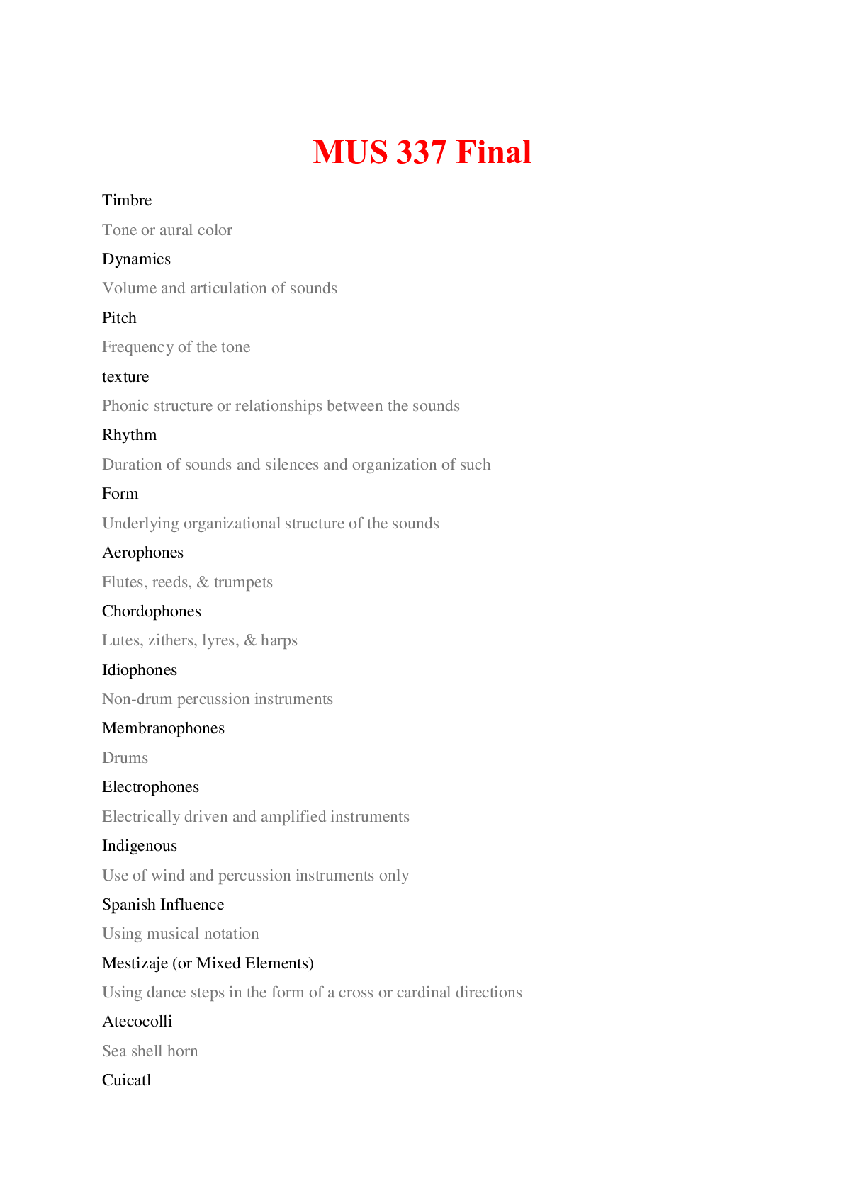
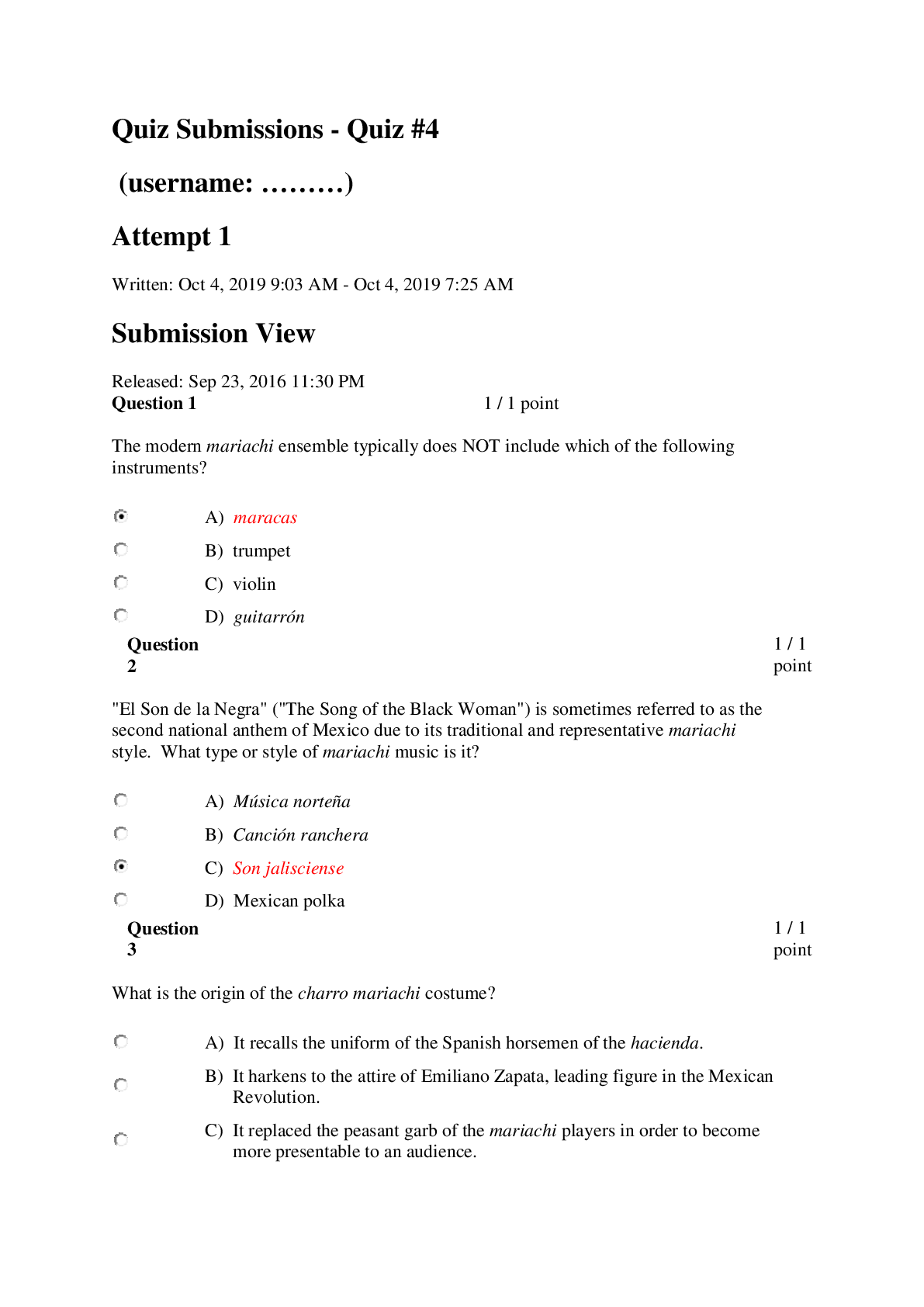


 Questions and Answers (latest Update), Correct, Download to Score A.png)
 Questions and Answers (latest Update), All Correct, Download to Score A.png)