Calculus > QUESTIONS & ANSWERS > Chapter 7: TECHNIQUES OF INTEGRATION. Work and Answers (All)
Chapter 7: TECHNIQUES OF INTEGRATION. Work and Answers
Document Content and Description Below
7.1 Integration by Parts 1. Let = , = 2 ⇒ = , = 1 22. Then by Equation 2, 2 = 1 22 − 1 22 = 1 2... 2 − 1 42 + . 2. Let = ln, = √ ⇒ = 1 , = 2 332. Then by Equation 2, √ln = 2 332 ln − 2 332 · 1 = 2 332 ln − 2 312 = 2 332 ln − 4 932 + . Note: A mnemonic device which is helpful for selecting when using integration by parts is the LIATE principle of precedence for : Logarithmic Inverse trigonometric Algebraic Trigonometric Exponential If the integrand has several factors, then we try to choose among them a which appears as high as possible on the list. For example, in 2 the integrand is 2, which is the product of an algebraic function () and an exponential function (2). Since Algebraic appears before Exponential, we choose = . Sometimes the integration turns out to be similar regardless of the selection of and , but it is advisable to refer to LIATE when in doubt. 3. Let = , = cos 5 ⇒ = , = 1 5 sin5. Then by Equation 2, cos5 = 1 5sin5 − 1 5 sin5 = 1 5sin5 + 25 1 cos5 + . 4. Let = , = 02 ⇒ = , = 01202. Then by Equation 2, 02 = 502 − 502 = 502 − 2502 + . 5. Let = , = −3 ⇒ = , = − 1 3−3. Then by Equation 2, −3 = − 1 3−3 − − 1 3−3 = − 1 3−3 + 1 3 −3 = − 1 3−3 − 1 9−3 + . 6. Let = − 1, = sin ⇒ = , = − 1 cos . Then by Equation 2, ( − 1) sin = −1 ( − 1) cos − −1 cos = −1 ( − 1) cos + 1 cos = − 1 ( − 1) cos + 1 2 sin + 7. First let = 2 + 2, = cos ⇒ = (2 + 2), = sin. Then by Equation 2, = (2 + 2)cos = (2 + 2)sin − (2 + 2) sin . Next let = 2 + 2, = sin ⇒ = 2, = −cos, so (2 + 2) sin = −(2 + 2) cos − −2cos = −(2 + 2) cos + 2 sin. Thus, = (2 + 2)sin + (2 + 2) cos − 2sin + . °c 2016 Cengage Learning. All Rights Reserved. May not be scanned, copied, or duplicated, or posted to a publicly accessible website, in whole or in part. 12 ¤ CHAPTER 7 TECHNIQUES OF INTEGRATION 8. First let = 2, = sin ⇒ = 2 , = − 1 cos. Then by Equation 2, = 2 sin = − 1 2 cos − − 2 cos . Next let = , = cos ⇒ = , = 1 sin, so cos = 1 sin − 1 sin = 1 sin + 12 cos . Thus, = − 1 2 cos + 2 1 sin + 12 cos + = −1 2 cos + 22 sin + 23 cos + . 9. Let = cos−1 , = ⇒ = √1−−12 , = . Then by Equation 2, cos−1 = cos−1 − √1−−2 = cos−1 − √1 1 2 = 1 = −−2 2, = cos−1 − 1 2 · 212 + = cos−1 − √1 − 2 + 10. Let = ln√, = ⇒ = √1 · 2√1 = 21 , = . Then by Equation 2, ln√ = ln√ − · 21 = ln√ − 1 2 = ln√ − 12 + . Note: We could start by using ln√ = 1 2 ln. 11. Let = ln, = 4 ⇒ = 1 , = 1 5 5. Then by Equation 2, 4 ln = 155 ln − 155 · 1 = 155 ln − 1 54 = 155 ln − 25 1 5 + . 12. Let = tan−1 2, = ⇒ = 2 1 + 42 , = . Then by Equation 2, tan−1 2 = tan−1 2 − 1 + 4 2 2 = tan−1 2 − 1 14 = 1 + 4 = 8 2, = tan−1 2 − 1 4 ln|| + = tan−1 2 − 1 4 ln(1 + 42) + 13. Let = , = csc2 ⇒ = , = −cot. Then by Equation 2, csc2 = −cot − −cot = −cot + cos sin = −cot + 1 = sin = cos , = −cot + ln|| + = −cot + ln|sin| + 14. Let = , = cosh ⇒ = , = 1 sinh. Then by Equation 2, cosh = 1sinh − 1 sinh = 1sinh − 12 cosh + . 15. First let = (ln)2, = ⇒ = 2ln · 1 , = . Then by Equation 2, = (ln)2 = (ln)2 − 2 ln · 1 = (ln)2 − 2 ln . Next let = ln, = ⇒ = 1 , = to get ln = ln − · (1) = ln − = ln − + 1. Thus, = (ln)2 − 2(ln − + 1) = (ln)2 − 2ln + 2 + , where = −21. °c 2016 Cengage Learning. All Rights Reserved. May not be scanned, copied, or duplicated, or posted to a publicly accessible website, in whole or in part.SECTION 7.1 INTEGRATION BY PARTS ¤ 3 16. 10 = 10− . Let = , = 10− ⇒ = , = −ln 10 10− . Then by Equation 2, 10− = −ln 10 10− − −ln 10 10− = 10−ln 10 − (ln 10)(ln 10) 10− + = −10 ln 10 − 10(ln 10) 1 2 + . 17. First let = sin3, = 2 ⇒ = 3cos3 , = 1 2 2. Then = 2 sin3 = 1 2 2 sin3 − 3 2 2 cos3 . Next let = cos3, = 2 ⇒ = −3sin3 , = 1 2 2 to get 2 cos3 = 1 2 2 cos 3 + 3 2 2 sin3 . Substituting in the previous formula gives = 1 2 2 sin3 − 3 4 2 cos3 − 9 4 2 sin3 = 1 2 2 sin3 − 3 4 2 cos 3 − 9 4 ⇒ 13 4 = 1 2 2 sin3 − 3 4 2 cos3 + 1. Hence, = 13 1 2(2sin3 − 3cos3) + , where = 13 4 1. 18. First let = −, = cos2 ⇒ = −− , = 1 2 sin2. Then = − cos2 = 1 2 − sin2 − 1 2 sin2 −− = 1 2 − sin2 + 1 2 − sin2 . Next let = −, = sin2 ⇒ = −− , = − 1 2 cos2, so − sin2 = − 1 2 − cos2 − − 1 2cos2−− = − 1 2 − cos2 − 1 2 − cos2 . So = 1 2 − sin2 + 1 2 − 1 2 − cos2 − 1 2 = 1 2 − sin2 − 1 4 − cos 2 − 1 4 ⇒ 5 4 = 1 2 − sin2 − 1 4 − cos2 +1 ⇒ = 4 5 1 2 − sin2 − 1 4 − cos 2 + 1 = 2 5 − sin2 − 1 5 − cos2 +. 19. First let = 3, = ⇒ = 32, = . Then 1 = 3 = 3 − 3 2. Next let 1 = 2, 1 = ⇒ 1 = 2 , 1 = . Then 2 = 2 − 2 . Finally, let 2 = , 2 = ⇒ 2 = , 2 = . Then = − = − + 1. Substituting in the expression for 2, we get 2 = 2 − 2( − + 1) = 2 − 2 + 2 − 21. Substituting the last expression for 2 into 1 gives 1 = 3 − 3(2 − 2 + 2 − 21) = 3 − 32 + 6 − 6 + , where = 61. 20. tan2 = (sec2 − 1) = sec2 − . Let = , = sec2 ⇒ = , = tan. Then by Equation 2, sec2 = tan − tan = tan − ln|sec|, and thus, tan2 = tan − ln|sec| − 1 2 2 + . 21. Let = 2, = 1 (1 + 2)2 ⇒ = ( · 22 + 2 · 1) = 2(2 + 1), = −2(1 + 2 1 ). Then by Equation 2, (1 + 2 2)2 = −2(1 + 2 2 ) + 1 2 21 + 2 (2 + 1) = −2(1 + 2 2 ) + 1 2 2 = −2(1 + 2 2 ) + 1 42 + . The answer could be written as 2 4(2 + 1) + . 22. First let = (arcsin)2, = ⇒ = 2 arcsin · √1 1− 2 , = . Then = (arcsin)2 = (arcsin)2 − 2 √arcsin 1 − 2 . To simplify the last integral, let = arcsin [ = sin], so °c 2016 Cengage Learning. All Rights Reserved. May not be scanned, copied, or duplicated, or posted to a publicly accessible website, in whole or in part.4 ¤ CHAPTER 7 TECHNIQUES OF INTEGRATION = √1 1− 2 , and √arcsin 1 − 2 = sin . To evaluate just the last integral, now let = , = sin ⇒ = , = −cos . Thus, sin = −cos + cos = −cos + sin + = −arcsin · √1 − 2 1 + + 1 [refer to the figure] Returning to , we get = (arcsin)2 + 2√1 − 2 arcsin − 2 + , where = −21. 23. Let = , = cos ⇒ = , = 1 sin. By (6), 012 cos = 1 sin1 02 − 012 1 sin = 21 − 0 − 1 −1 cos1 02 = 1 2 + 1 2 (0 − 1) = 1 2 − 1 2 or − 2 22 24. First let = 2 + 1, = − ⇒ = 2 , = −−. By (6), 01(2 + 1)− = −(2 + 1)−1 0 + 01 2− = −2−1 + 1 + 201 − . Next let = , = − ⇒ = , = −−. By (6) again, 01 − = −−1 0 + 01 − = −−1 + −−1 0 = −−1 − −1 + 1 = −2−1 + 1. So 01(2 + 1)− = −2−1 + 1 + 2(−2−1 + 1) = −2−1 + 1 − 4−1 + 2 = −6−1 + 3. 25. Let = , = sinh ⇒ = , = cosh. By (6), 02 sinh = cosh2 0 − 02 cosh = 2 cosh 2 − 0 − sinh2 0 = 2 cosh 2 − sinh 2. 26. Let = ln, = 2 ⇒ = 1 , = 1 33. By (6), 12 2 ln = 1 33 ln2 1 − 12 1 32 = 8 3 ln 2 − 0 − 1 932 1 = 8 3 ln 2 − 8 9 − 1 9 = 8 3 ln 2 − 7 9 . 27. Let = ln, = 1 2 ⇒ = 1 , = −1 . By (6), 15 ln2 = −1 ln5 1 − 15 −12 = − 1 5 ln 5 − 0 − 1 5 1 = − 1 5 ln 5 − 1 5 − 1 = 4 5 − 1 5 ln 5. 28. First let = 2, = sin 2 ⇒ = 2 , = − 1 2 cos 2. By (6), 02 2 sin 2 = − 1 22 cos 22 0 + 02 cos 2 = −22 + 02 cos 2 . Next let = , = cos 2 ⇒ = , = 1 2 sin 2. By (6) again, 02 cos 2 = 1 2sin 22 0 − 02 1 2 sin 2 = 0 − − 1 4 cos 22 0 = 1 4 − 1 4 = 0. Thus, 02 2 sin 2 = −22. 29. sin 2 = 2 sin cos, so 0 sin cos = 1 2 0 sin 2 . Let = , = sin 2 ⇒ = , = − 1 2 cos 2. By (6), 1 2 0 sin 2 = 1 2− 1 2cos 2 0 − 1 2 0 − 1 2 cos 2 = − 1 4 − 0 + 1 4 1 2 sin 2 0 = −4 . °c 2016 Cengage Learning. All Rights Reserved. May not be scanned, copied, or duplicated, or posted to a publicly accessible website, in whole or in part.SECTION 7.1 INTEGRATION BY PARTS ¤ 5 30. Let = arctan(1), = ⇒ = 1 1 + (1)2 · −1 2 = −2 + 1, = . By (6), 1√3 arctan1 = arctan1√ 1 3 + 1√3 2 + 1 = √3 6 − 1 · 4 + 12ln(2 + 1)√ 1 3 = √3 6 − 4 + 1 2 (ln 4 − ln 2) = √3 6 − 4 + 1 2 ln 4 2 = √3 6 − 4 + 1 2 ln 2 31. Let = , = − ⇒ = , = −−. By (6), 15 = 15 − = −−5 1 − 15 −− = −5−5 + −1 − −5 1 = −5−5 + −1 − (−5 − −1) = 2−1 − 6−5 32. Let = (ln)2, = −3 ⇒ = 2ln = − 1 2−2. By (6), = 12 (ln3)2 = −(ln 22)2 2 1 + 12 ln 3 . Now let = ln, = −3 ⇒ = 1 , = − 1 2−2. Then 12 ln3 = −ln 22 2 1 + 1 2 12 −3 = − 1 8 ln 2 + 0 + 1 2 − 212 2 1 = − 1 8 ln 2 + 1 2 − 1 8 + 1 2 = 16 3 − 1 8 ln 2. Thus = − 1 8 (ln 2)2 + 0 + 16 3 − 1 8 ln 2 = − 1 8 (ln 2)2 − 1 8 ln 2 + 16 3 . 33. Let = ln(cos), = sin ⇒ = 1 cos (−sin), = −cos. By (6), 03 sin ln(cos) = − cos ln(cos) 0 3 − 03 sin = − 1 2 ln 1 2 − 0 − − cos 0 3 = − 1 2 ln 1 2 + 1 2 − 1 = 1 2 ln 2 − 1 2 34. Let = 2, = √4 + 2 ⇒ = 2 , = √4 + 2. By (6), 01 √4 + 3 2 = 2√4 + 2 1 0 − 201 4 + 2 = √5 − 2 3(4 + 2)321 0 = √5 − 2 3(5)32 + 2 3(8) = √51 − 10 3 + 16 3 = 16 3 − 7 3√5 35. Let = (ln)2, = 4 ⇒ = 2 ln , = 5 5 . By (6), 12 4(ln)2 = 55 (ln)22 1 − 212 54 ln = 32 5 (ln 2)2 − 0 − 212 54 ln . Let = ln, = 4 5 ⇒ = 1 , = 5 25 . Then 12 54 ln = 255 ln2 1 − 12 254 = 32 25 ln 2 − 0 − 125 5 2 1 = 32 25 ln 2 − 125 32 − 125 1 . So 12 4(ln)2 = 32 5 (ln 2)2 − 2 32 25 ln 2 − 125 31 = 32 5 (ln 2)2 − 64 25 ln 2 + 125 62 . °c 2016 Cengage Learning. All Rights Reserved. May not be scanned, copied, or duplicated, or posted to a publicly accessible website, in whole or in part.6 ¤ CHAPTER 7 TECHNIQUES OF INTEGRATION 36. Let = sin( − ), = ⇒ = −cos( − ), = . Then = 0 sin( − ) = sin( − ) 0 + 0 cos( − ) = sin0 − 0 sin + 1. For 1, let = cos( − ), = ⇒ = sin( − ), = . So 1 = cos( − ) 0 − 0 sin( − ) = cos0 − 0 cos − . Thus, = −sin + − cos − ⇒ 2 = − cos − sin ⇒ = 1 2( − cos − sin). 37. Let = √, so that 2 = and 2 = . Thus, √ = (2). Now use parts with = , = , = , and = to get 2 = 2 − 2 = 2 − 2 + = 2√ √ − 2√ + . 38. Let = ln, so that = and = . Thus, cos(ln) = cos · = . Now use parts with = cos, = , = −sin , and = to get cos = cos − − sin = cos + sin . Now use parts with = sin, = , = cos , and = to get sin = sin − cos . Thus, = cos + sin − ⇒ 2 = cos + sin ⇒ = 1 2 cos + 1 2 sin + = 1 2cos(ln) + 1 2sin(ln) + . 39. Let = 2, so that = 2 . Thus, √√/2 3 cos2 = √√/2 2 cos2 · 1 2(2 ) = 1 2 /2 cos . Now use parts with = , = cos , = , = sin to get 1 2 /2 cos = 1 2 sin /2 − /2 sin = 1 2 sin + cos /2 = 1 2 ( sin + cos) − 1 2 2 sin 2 + cos 2 = 1 2( · 0 − 1) − 1 2 2 · 1 + 0 = − 1 2 − 4 40. Let = cos, so that = −sin . Thus, 0 cos sin 2 = 0 cos (2 sin cos ) = 1−1 · 2(−) = 2−11 . Now use parts with = , = , = , = to get 2−11 = 21 −1 − −11 = 21 + −1 − 1 −1 = 2( + −1 − [1 − −1]) = 2(2−1) = 4. 41. Let = 1 + so that = . Thus, ln(1 + ) = ( − 1) ln . Now use parts with = ln = ( − 1), = 1 , = 1 22 − to get ( − 1) ln = 1 22 − ln − 1 2 − 1 = 1 2( − 2) ln − 1 42 + + = 1 2 (1 + )( − 1) ln(1 + ) − 1 4(1 + )2 + 1 + + , which can be written as 1 2(2 − 1) ln(1 + ) − 1 42 + 1 2 + 3 4 + . 42. Let = ln, so that = 1 . Thus, arcsin(ln ) = arcsin . Now use parts with = arcsin, = , = 11− 2 , and = to get arcsin = arcsin − 1− 2 = arcsin + 1 − 2 + = (ln)arcsin(ln) + 1 − (ln)2 + . °c 2016 Cengage Learning. All Rights Reserved. May not be scanned, copied, or duplicated, or posted to a publicly accessible website, in whole or in part.SECTION 7.1 INTEGRATION BY PARTS ¤ 7 43. Let = , = −2 ⇒ = , = − 1 2−2. Then −2 = − 1 2−2 + 1 2−2 = − 1 2−2 − 1 4−2 + . We see from the graph that this is reasonable, since has a minimum where changes from negative to positive. Also, increases where is positive and decreases where is negative. 44. Let = ln, = 32 ⇒ = 1 , = 2 552. Then 32 ln = 2 552 ln − 2 5 32 = 2 552 ln − 2 5 2 52 + = 2 5 52 ln − 4 2552 + We see from the graph that this is reasonable, since has a minimum where changes from negative to positive. 45. Let = 1 22, = 2 √1 + 2 ⇒ = , = 2 3(1 + 2)32. Then 3 √1 + 2 = 1 22 2 3(1 + 2)32 − 2 3 (1 + 2)32 = 1 3 2(1 + 2)32 − 2 3 · 2 5 · 1 2(1 + 2)52 + = 1 3 2(1 + 2)32 − 15 2 (1 + 2)52 + We see from the graph that this is reasonable, since increases where is positive and decreases where is negative. Note also that is an odd function and is an even function. Another method: Use substitution with = 1 + 2 to get 1 5(1 + 2)52 − 1 3(1 + 2)32 + . 46. First let = 2, = sin2 ⇒ = 2 , = − 1 2 cos2. Then = 2 sin2 = − 1 22 cos2 + cos2 . Next let = , = cos2 ⇒ = , = 1 2 sin2, so cos2 = 1 2sin2 − 1 2 sin2 = 1 2sin2 + 1 4 cos2 + . Thus, = − 1 22 cos 2 + 1 2sin2 + 1 4 cos2 + . We see from the graph that this is reasonable, since increases where is positive and decreases where is negative. Note also that is an odd function and is an even function. 47. (a) Take = 2 in Example 6 to get sin2 = −12 cossin + 12 1 = 2 − sin2 4 + . (b) sin4 = − 1 4 cos sin3 + 3 4 sin2 = − 1 4 cossin3 + 3 8 − 16 3 sin2 + . 48. (a) Let = cos−1 , = cos ⇒ = −( − 1)cos−2 sin , = sin in (2): cos = cos−1 sin + ( − 1) cos−2 sin2 = cos−1 sin + ( − 1) cos−2 (1 − cos2 ) = cos−1 sin + ( − 1) cos−2 − ( − 1) cos [continued] °c 2016 Cengage Learning. All Rights Reserved. May not be scanned, copied, or duplicated, or posted to a publicly accessible website, in whole or in part.8 ¤ CHAPTER 7 TECHNIQUES OF INTEGRATION Rearranging terms gives cos = cos−1 sin + ( − 1) cos−2 or cos = 1 cos−1 sin + − 1 cos−2 (b) Take = 2 in part (a) to get cos2 = 1 2 cos sin + 1 2 1 = 2 + sin 2 4 + . (c) cos4 = 1 4 cos3 sin + 3 4 cos2 = 1 4 cos3 sin + 3 8 + 16 3 sin 2 + 49. (a) From Example 6, sin = −1 cos sin−1 + − 1 sin−2 . Using (6), 02 sin = −cos sin −1 0 2 + − 1 02 sin−2 = (0 − 0) + − 1 02 sin−2 = − 1 02 sin−2 (b) Using = 3 in part (a), we have 02 sin3 = 2 3 02 sin = − 2 3 cos 0 2 = 2 3. Using = 5 in part (a), we have 02 sin5 = 4 5 02 sin3 = 4 5 · 2 3 = 15 8 . (c) The formula holds for = 1 (that is, 2 + 1 = 3) by (b). Assume it holds for some ≥ 1. Then 02 sin2+1 = 3 ·25··47·· · · · · 6 · · · · · (2(2 + 1) ) . By Example 6, 02 sin2+3 = 22 + 2 + 3 02 sin2+1 = 2 2 + 2 + 3 · 3 ·25··47·· · · · · 6 · · · · · (2(2 + 1) ) = 2 · 4 · 6 · · · · · (2)[2 ( + 1)] 3 · 5 · 7 · · · · · (2 + 1)[2 ( + 1) + 1], so the formula holds for = + 1. By induction, the formula holds for all ≥ 1. 50. Using Exercise 49(a), we see that the formula holds for = 1, because 02 sin2 = 1 2 02 1 = 1 2 0 2 = 1 2 · 2 . Now assume it holds for some ≥ 1. Then 02 sin2 = 1 ·23··45·· · · · · 6 · · · · · (2(2 −)1) 2 . By Exercise 49(a), 02 sin2(+1) = 22 + 1 + 2 02 sin2 = 2 2 + 1 + 2 · 1 ·23··45·· · · · · 6 · · · · · (2(2 −)1) 2 = 1 · 3 · 5 · · · · · (2 − 1)(2 + 1) 2 · 4 · 6 · · · · · (2)(2 + 2) · 2 , so the formula holds for = + 1. By induction, the formula holds for all ≥ 1. 51. Let = (ln), = ⇒ = (ln)−1(), = . By Equation 2, (ln) = (ln) − (ln)−1() = (ln) − (ln)−1 . 52. Let = , = ⇒ = −1 , = . By Equation 2, = − −1 . °c 2016 Cengage Learning. All Rights Reserved. May not be scanned, copied, or duplicated, or posted to a publicly accessible website, in whole or in part.SECTION 7.1 INTEGRATION BY PARTS ¤ 9 53. tan = tan−2 tan2 = tan−2 (sec2 − 1) = tan−2 sec2 − tan−2 = − tan−2 . Let = tan−2 , = sec2 ⇒ = ( − 2) tan−3 sec2 , = tan. Then, by Equation 2, = tan−1 − ( − 2) tan−2 sec2 1 = tan−1 − ( − 2) ( − 1) = tan−1 = tan−1 − 1 Returning to the original integral, tan = tan−1 − 1 − tan−2 . 54. Let = sec−2 , = sec2 ⇒ = ( − 2) sec−3 sec tan , = tan. Then, by Equation 2, sec = tan sec−2 − ( − 2) sec−2 tan2 = tan sec−2 − ( − 2) sec−2 (sec2 − 1) = tan sec−2 − ( − 2) sec + ( − 2) sec−2 so ( − 1) sec = tan sec−2 + ( − 2) sec−2 . If − 1 6= 0, then sec = tansec − 1−2 + −− 2 1 sec−2 . 55. By repeated applications of the reduction formula in Exercise 51, (ln)3 = (ln)3 − 3 (ln)2 = (ln)3 − 3(ln)2 − 2 (ln)1 = (ln)3 − 3(ln)2 + 6(ln)1 − 1 (ln)0 = (ln)3 − 3(ln)2 + 6ln − 6 1 = (ln)3 − 3(ln)2 + 6ln − 6 + 56. By repeated applications of the reduction formula in Exercise 52, 4 = 4 − 4 3 = 4 − 43 − 3 2 = 4 − 43 + 122 − 2 1 = 4 − 43 + 122 − 241 − 0 = 4 − 43 + 122 − 24+ 24 + or (4 − 43 + 122 − 24 + 24) + 57. The curves = 2 ln and = 4 ln intersect when 2 ln = 4 ln ⇔ 2 ln − 4ln = 0 ⇔ (2 − 4) ln = 0 ⇔ = 1 or 2 [since 0]. For 1 2, 4ln 2 ln Thus, area = 12(4 ln − 2 ln) = 12[(4 − 2)ln]. Let = ln, = (4 − 2) ⇒ = 1 , = 4 − 1 33. Then area = (ln)4 − 1 332 1 − 12 4 − 1 331 = (ln 2) 16 3 − 0 − 12 4 − 1 32 = 16 3 ln 2 − 4 − 1 932 1 = 16 3 ln 2 − 64 9 − 35 9 = 16 3 ln 2 − 29 9 °c 2016 Cengage Learning. All Rights Reserved. May not be scanned, copied, or duplicated, or posted to a publicly accessible website, in whole or in part.10 ¤ CHAPTER 7 TECHNIQUES OF INTEGRATION 58. The curves = 2− and = − intersect when 2− = − ⇔ 2 − = 0 ⇔ ( − 1) = 0 ⇔ = 0 or 1. For 0 1, − 2−. Thus, area = 01(− − 2−) = 01( − 2)− . Let = − 2, = − ⇒ = (1 − 2), = −−. Then area = ( − 2)(−−)1 0 − 01[−−(1 − 2)] = 0 + 01(1 − 2)− . Now let = 1 − 2, = − ⇒ = −2, = −−. Now area = (1 − 2)(−−)1 0 − 01 2− = −1 + 1 − −2−1 0 = −1 + 1 + 2(−1 − 1) = 3−1 − 1. 59. The curves = arcsin 1 2 and = 2 − 2 intersect at = ≈ −175119 and = ≈ 117210. From the figure, the area bounded by the curves is given by = [(2 − 2) − arcsin 1 2 ] = 2 − 1 3 3 − arcsin 1 2 . Let = arcsin 1 2 , = ⇒ = 1 −1 1 2 2 · 1 2 , = . Then = 2 − 133 − arcsin1 2 − 21− 1 4 2 = 2 − 1 3 3 − arcsin 1 2 − 21 − 1 42 ≈ 399926 60. The curves = ln( + 1) and = 3 − 2 intersect at = 0 and = ≈ 192627. From the figure, the area bounded by the curves is given by = 0[(3−2)−ln(+1)] = 3 2 2 − 1 33 0 −0 ln(+1). Let = ln( + 1), = ⇒ = 1 + 1 , = 1 2 2. Then = 322 − 133 0 − 1 22 ln( + 1) 0 − 12 0 + 1 2 = 322 − 133 0 − 1 22 ln( + 1) 0 + 12 0 − 1 + + 1 1 = 3 2 2 − 1 33 − 1 2 2 ln( + 1) + 1 42 − 1 2 + 1 2 ln| + 1| 0 ≈ 169260 61. Volume = 01 2cos(2). Let = , = cos(2) ⇒ = , = 2 sin(2). = 2 2 sin 2 1 0 − 2 · 2 01 sin 2 = 22 − 0 − 4−2 cos 2 1 0 = 4 + 8 (0 − 1) = 4 − 8 . 62. Volume = 01 2( − −) = 2 01( − −) = 201 − 01 − [both integrals by parts] = 2( − ) − −− − − 1 0 = 2[2 − 0] = 4 °c 2016 Cengage Learning. All Rights Reserved. May not be scanned, copied, or duplicated, or posted to a publicly accessible website, in whole or in part.SECTION 7.1 INTEGRATION BY PARTS ¤ 11 63. Volume = −01 2(1 − )− . Let = 1 − , = − ⇒ = − , = −−. = 2(1 − )(−−)0 −1 − 2 −01 − = 2( − 1)(−) + −0 −1 = 2−0 −1 = 2(0 + ) = 2. 64. = ⇔ = ln. Volume = 13 2 ln . Let = ln, = ⇒ = 1 , = 1 22. = 2 1 22 ln3 1 − 2 13 1 2 = 2 1 22 ln − 1 423 1 = 2 9 2 ln 3 − 9 4 − 0 − 1 4 = 2 9 2 ln 3 − 2 = (9 ln 3 − 4) 65. (a) Use shells about the -axis: = 12 2ln = ln = 1 , , == 1 2 2 = 2 1 22 ln2 1 − 12 1 2 = 2(2 ln 2 − 0) − 1 422 1 = 22ln2 − 3 4 (b) Use disks about the -axis: = 12 (ln)2 = (ln = 2 ln)2·, 1 , == = (ln)22 1 − 12 2ln = ln = 1 , , == = 2(ln 2)2 − 2ln2 1 − 12 = 2(ln 2)2 − 4ln2 + 22 1 = [2(ln 2)2 − 4ln2 + 2] = 2[(ln 2)2 − 2ln2 + 1] 66. ave = 1 − () = 41− 0 04 sec2 == , , = tan = sec2 = 4 tan 0 4 − 04 tan = 4 4 − ln|sec| 0 4 = 4 4 − ln√2 = 1 − 4 ln√2 or 1 − 2 ln 2 67. () = 0 sin 1 22 ⇒ () = 0 sin 1 22 . Let = 0 sin 1 22 = (), = ⇒ = sin 1 22 , = . Thus, () = () − sin 1 22 = () − sin 1 == 1 2 2 = () + 1 cos + = () + 1 cos 1 22 + 68. The rocket will have height = 060 () after 60 seconds. = 060 − − ln − = − 1 2260 0 − 060 ln( − ) − 060 ln = −(1800) + (ln)(60) − 060 ln( − ) Let = ln( − ), = ⇒ = 1 − (−), = . Then °c 2016 Cengage Learning. All Rights Reserved. May not be scanned, copied, or duplicated, or posted to a publicly accessible website, in whole or in part.12 ¤ CHAPTER 7 TECHNIQUES OF INTEGRATION 060 ln( − ) = ln( − )60 0 + 060 − = 60 ln( − 60) + 060−1 + − = 60 ln( − 60) + − − ln( − )60 0 = 60 ln( − 60) − 60 − ln( − 60) + ln So = −1800 + 60 ln − 60 ln( − 60) + 60 + ln( − 60) − ln. Substituting = 98, = 30,000, = 160, and = 3000 gives us ≈ 14,844 m. 69. Since () 0 for all , the desired distance is () = 0 () = 0 2− . First let = 2, = − ⇒ = 2 , = −−. Then () = −2− 0 + 20 − . Next let = , = − ⇒ = , = −−. Then () = −2− + 2−− 0 + 0 − = −2− + 2−− + 0 + −− 0 = −2− + 2(−− − − + 1) = −2− − 2− − 2− + 2 = 2 − −(2 + 2 + 2) meters 70. Suppose (0) = (0) = 0 and let = (), = 00() ⇒ = 0(), = 0(). Then 0 ()00() = ()0() 0 − 0 0()0() = ()0() − 0 0()0(). Now let = 0(), = 0() ⇒ = 00() and = (), so 0 0()0() = 0()() 0 − 0 00()() = 0()() − 0 00()(). Combining the two results, we get 0 ()00() = ()0() − 0()() + 0 00()(). 71. For = 14 00(), let = , = 00() ⇒ = , = 0(). Then = 0()4 1 − 14 0() = 4 0(4) − 1 · 0(1) − [(4) − (1)] = 4 · 3 − 1 · 5 − (7 − 2) = 12 − 5 − 5 = 2. We used the fact that 00 is continuous to guarantee that exists. 72. (a) Take () = and 0() = 1 in Equation 1. (b) By part (a), () = () − () − 0(). Now let = (), so that = () and = 0(). Then 0() = (()) (). The result follows. (c) Part (b) says that the area of region is = () − () − (()) () = (area of rectangle ) − (area of rectangle ) − (area of region ) °c 2016 Cengage Learning. All Rights Reserved. May not be scanned, copied, or duplicated, or posted to a publicly accessible website, in whole or in part.SECTION 7.1 INTEGRATION BY PARTS ¤ 13 (d) We have () = ln, so −1() = , and since = −1, we have () = . By part (b), 1 ln = ln − 1ln1 − ln 1 ln = − 01 = − 1 0 = − ( − 1) = 1. 73. Using the formula for volumes of rotation and the figure, we see that Volume = 0 2 − 0 2 − [()]2 = 2 − 2 − [()]2 . Let = (), which gives = 0() and () = , so that = 2 − 2 − 2 0(). Now integrate by parts with = 2, and = 0() ⇒ = 2 , = (), and 2 0() = 2 () − 2 () = 2 () − 2 () − 2 (), but () = and () = ⇒ = 2 − 2 − 2 − 2 − 2 () = 2 (). 74. (a) We note that for 0 ≤ ≤ 2 , 0 ≤ sin ≤ 1, so sin2+2 ≤ sin2+1 ≤ sin2 . So by the second Comparison Property of the Integral, 2+2 ≤ 2+1 ≤ 2. (b) Substituting directly into the result from Exercise 50, we get 2+2 2 = 1 · 3 · 5 · · · · · [2( + 1) − 1] 2 · 4 · 6 · · · · · [2( + 1)] 2 1 · 3 · 5 · · · · · (2 − 1) 2 · 4 · 6 · · · · · (2) 2 = 2( + 1) − 1 2( + 1) = 2 + 1 2 + 2 (c) We divide the result from part (a) by 2. The inequalities are preserved since 2 is positive: 2+2 2 ≤ 22+1 ≤ 2 2 . Now from part (b), the left term is equal to 2 + 1 2 + 2 , so the expression becomes 2 + 1 2 + 2 ≤ 2+1 2 ≤ 1. Now lim →∞ 2 + 1 2 + 2 = lim →∞ 1 = 1, so by the Squeeze Theorem, lim →∞ 2+1 2 = 1. (d) We substitute the results from Exercises 49 and 50 into the result from part (c): 1 = lim →∞ 2+1 2 = lim →∞ 2 · 4 · 6 · · · · · (2) 3 · 5 · 7 · · · · · (2 + 1) 1 · 3 · 5 · · · · · (2 − 1) 2 · 4 · 6 · · · · · (2) 2 = lim →∞ 3 ·25··47·· · · · · 6 · · · · · (2(2 + 1) ) 1 ·23··45·· · · · · 6 · · · · · (2(2 −)1)2 = lim →∞ 2 1 · 2 3 · 4 3 · 4 5 · 6 5 · 6 7 · · · · · 2 2 − 1 · 2 2 + 1 · 2 [rearrange terms] Multiplying both sides by 2 gives us the Wallis product: 2 = 2 1 · 2 3 · 4 3 · 4 5 · 6 5 · 6 7 · · · · (e) The area of the th rectangle is . At the 2th step, the area is increased from 2 − 1 to 2 by multiplying the width by 2 2 − 1 , and at the (2 + 1)th step, the area is increased from 2 to 2 + 1 by multiplying the height by 2 + 1 2 . These two steps multiply the ratio of width to height by 2 2 − 1 and 1 (2 + 1)(2) = 2 2 + 1 respectively. So, by part (d), the limiting ratio is 2 1 · 2 3 · 4 3 · 4 5 · 6 5 · 6 7 · · · · = 2 . °c 2016 Cengage Learning. All Rights Reserved. May not be scanned, copied, or duplicated, or posted to a publicly accessible website, in whole or in part.14 ¤ CHAPTER 7 TECHNIQUES OF INTEGRATION 7.2 Trigonometric Integrals The symbols =s and =c indicate the use of the substitutions { = sin = cos } and { = cos = −sin }, respectively. 1. sin2 cos3 = sin2 cos2 cos = sin2 (1 − sin2 ) cos s= 2(1 − 2) = (2 − 4) = 1 33 − 1 55 + = 1 3 sin3 − 1 5 sin5 + 2. sin3 cos4 = sin2 cos4 sin = (1 − cos2 ) cos4 sin c= (1 − 2)4(−) = (6 − 4) = 1 77 − 1 55 + = 1 7 cos7 − 1 5 cos5 + 3. 02 sin7 cos5 = 02 sin7 cos4 cos = 02 sin7 (1 − sin2 )2 cos s= 01 7(1 − 2)2 = 01 7(1 − 22 + 4) = 01(7 − 29 + 11) = 1 88 − 1 510 + 12 1 121 0 = 18 − 1 5 + 12 1 − 0 = 15 −120 24 + 10 = 120 1 4. 02 sin5 = 02 sin4 sin = 02(1 − cos2 )2 sin =c 10(1 − 2)2(−) = 01(1 − 22 + 4) = − 233 + 1 551 0 = 1 − 23 + 15 − 0 = 15 −15 10 + 3 = 15 8 5. sin5(2)cos2(2) = sin4(2) cos2(2) sin(2) = [1 − cos2(2)]2 cos2(2) sin(2) = (1 − 2)2 2 − 1 2 [ = cos(2), = −2sin(2)] = − 1 2 (4 − 22 + 1)2 = − 1 2 (6 − 24 + 2) = − 1 2 1 77 − 2 55 + 1 33 + = − 14 1 cos7(2) + 1 5 cos5(2) − 1 6 cos3(2) + 6. cos5(2) = cos4(2) cos(2) = [1 − sin2(2)]2 cos(2) = 1 2(1 − 2)2 = sin(2), = 2cos(2) = 1 2 (4 − 22 + 1) = 1 2( 1 55 − 2 33 + ) + = 10 1 sin5(2) − 1 3 sin3(2) + 1 2 sin(2) + 7. 02 cos2 = 02 1 2(1 + cos 2) [half-angle identity] = 1 2 + 1 2 sin 2 0 2 = 1 2 2 + 0 − (0 + 0) = 4 8. 02 sin2 1 3 = 02 1 2 1 − cos2 · 1 3 [half-angle identity] = 1 2 − 3 2 sin2 32 0 = 1 22 − 3 2−√23 − 0 = + 3 8 √3 9. 0 cos4(2) = 0[cos2(2)]2 = 0 1 2(1 + cos(2 · 2))2 [half-angle identity] = 1 4 0[1 + 2 cos 4 + cos2(4)] = 1 4 0[1 + 2 cos 4 + 1 2(1 + cos 8)] = 1 4 0 3 2 + 2 cos 4 + 1 2 cos 8 = 1 4 3 2 + 1 2 sin 4 + 16 1 sin 8 0 = 1 4 3 2 + 0 + 0 − 0 = 3 8 10. 0 sin2 cos4 = 1 4 0(4 sin2 cos2 )cos2 = 1 4 0(2 sin cos )2 1 2(1 + cos 2) = 1 8 0(sin 2)2(1 + cos 2) = 1 8 0(sin2 2 + sin2 2 cos 2) = 1 8 0 sin2 2 + 1 8 0 sin2 2 cos 2 = 1 8 0 12(1 − cos 4) + 1 8 1 3 · 1 2 sin3 2 0 = 1 16 − 1 4 sin 4 0 + 1 8(0 − 0) = 16 1 [( − 0) − 0] = 16 °c 2016 Cengage Learning. All Rights Reserved. May not be scanned, copied, or duplicated, or posted to a publicly accessible website, in whole or in part.SECTION 7.2 TRIGONOMETRIC INTEGRALS ¤ 15 11. 02 sin2 cos2 = 02 1 4(4 sin2 cos2 ) = 02 14(2 sin cos)2 = 1 4 02 sin2 2 = 1 4 02 1 2(1 − cos 4) = 1 8 02(1 − cos 4) = 1 8 − 1 4 sin 4 0 2 = 1 8 2 = 16 12. 02(2 − sin)2 = 02(4 − 4sin + sin2 ) = 02 4 − 4sin + 1 2(1 − cos 2) = 02 9 2 − 4sin − 1 2 cos 2 = 9 2 + 4 cos − 1 4 sin 2 0 2 = 94 + 0 − 0 − (0 + 4 − 0) = 9 4 − 4 13. √cos sin3 = √cos sin2 sin = (cos)12(1 − cos2 )sin c= 12(1 − 2)(−) = (52 − 12) = 2 7 72 − 2 332 + = 2 7(cos)72 − 2 3(cos)32 + 14. sin2(1 2 ) = sin2 (−) = 1 , = −12 = − 1 2(1 − cos 2) = −12 − 12 sin 2 + = −21 + 1 4 sin2 + 15. cot cos2 = cos sin (1 − sin2 ) s= 1 −2 = 1 − = ln|| − 1 22 + = ln|sin| − 1 2 sin2 + 16. tan2 cos3 = cos sin22 cos3 = sin2 cos =s 2 = 1 33 + = 1 3 sin3 + 17. sin2 sin 2 = sin2 (2 sin cos ) =s 23 = 1 24 + = 1 2 sin4 + 18. sin cos 1 2 = sin2 · 1 2cos 1 2 = 2sin 1 2cos2 1 2 = 22 (−2) [ = cos 1 2 , = − 1 2 sin 1 2 ] = − 4 3 3 + = − 4 3 cos3 1 2 + 19. sin2 = 1 2(1 − cos 2) = 1 2 ( − cos 2) = 1 2 − 1 2 cos 2 = 1 2 1 22 − 1 2 1 2sin 2 − 1 2 sin 2 == , , == cos 2 1 2 sin 2 = 1 4 2 − 1 4sin 2 + 1 2 − 1 4 cos 2 + = 1 42 − 1 4sin 2 − 1 8 cos 2 + 20. = sin3 . First, evaluate sin3 = (1 − cos2 ) sin =c (1 − 2)(−) = (2 − 1) = 1 33 − + 1 = 1 3 cos3 − cos + 1. Now for , let = , = sin3 ⇒ = , = 1 3 cos3 − cos, so = 1 3cos3 − cos − 1 3 cos3 − cos = 1 3cos3 − cos − 1 3 cos3 + sin = 1 3 cos3 − cos − 1 3(sin − 1 3 sin3 ) + sin + [by Example 1] = 1 3 cos3 − cos + 2 3 sin + 1 9 sin3 + 21. tan sec3 = tan sec sec2 = 2 [ = sec , = sec tan ] = 1 3 3 + = 1 3 sec3 + °c 2016 Cengage Learning. All Rights Reserved. May not be scanned, copied, or duplicated, or posted to a publicly accessible website, in whole or in part.16 ¤ CHAPTER 7 TECHNIQUES OF INTEGRATION 22. tan2 sec4 = tan2 sec2 sec2 = tan2 (tan2 + 1) sec2 = 2(2 + 1) [ = tan , = sec2 ] = (4 + 2) = 1 5 5 + 1 3 3 + = 1 5 tan5 + 1 3 tan3 + 23. tan2 = (sec2 − 1) = tan − + 24. (tan2 + tan4 ) = tan2 (1 + tan2 ) = tan2 sec2 = 2 [ = tan , = sec2 ] = 1 3 3 + = 1 3 tan3 + 25. Let = tan. Then = sec2 , so tan4sec6 = tan4sec4(sec2 ) = tan4(1 + tan2)2 (sec2 ) = 4(1 + 2)2 = (8 + 26 + 4) = 1 9 9 + 2 7 7 + 1 5 5 + = 1 9 tan9 + 2 7 tan7 + 1 5 tan5 + 26. 04 sec6 tan6 = 04 tan6 sec4 sec2 = 04 tan6 (1 + tan2 )2 sec2 = 01 6(1 + 2)2 = tan = sec2 , = 01 6(4 + 22 + 1) = 01(10 + 28 + 6) = 11 1 11 + 2 9 9 + 1 7 71 0 = 11 1 + 2 9 + 1 7 = 63 + 154 + 99 693 = 316 693 27. tan3 sec = tan2 sec tan = (sec2 − 1) sec tan = (2 − 1) [ = sec, = sec tan ] = 1 3 3 − + = 1 3 sec3 − sec + 28. Let = sec, so = sectan . Thus, tan5sec3 = tan4sec2(sectan) = (sec2 − 1)2 sec2(sectan ) = (2 − 1)22 = (6 − 24 + 2) = 1 7 7 − 2 5 5 + 1 3 3 + = 1 7 sec7 − 2 5 sec5 + 1 3 sec3 + 29. tan3 sec6 = tan3 sec4 sec2 = tan3 (1 + tan2 )2 sec2 = 3(1 + 2)2 = tan = sec2 , = 3(4 + 22 + 1) = (7 + 25 + 3) = 1 8 8 + 1 3 6 + 1 4 4 + = 1 8 tan8 + 1 3 tan6 + 1 4 tan4 + 30. 04 tan4 = 04 tan2 (sec2 − 1) = 04 tan2 sec2 − 04 tan2 = 01 2 [ = tan ] − 04(sec2 − 1) = 1 3 31 0 − tan − 0 4 = 1 3 − 1 − 4 − 0 = 4 − 2 3 31. tan5 = (sec2 − 1)2 tan = sec4 tan − 2 sec2 tan + tan = sec3 sec tan − 2 tan sec2 + tan = 1 4 sec4 − tan2 + ln|sec| + [or 1 4 sec4 − sec2 + ln|sec| + ] °c 2016 Cengage Learning. All Rights Reserved. May not be scanned, copied, or duplicated, or posted to a publicly accessible website, in whole or in part.SECTION 7.2 TRIGONOMETRIC INTEGRALS ¤ 17 32. tan2 sec = (sec2 − 1) sec = sec3 − sec = 1 2 (sec tan + ln|sec + tan|) − ln|sec + tan| + [by Example 8 and (1)] = 1 2 (sec tan − ln|sec + tan|) + 33. Let = = sec tan ⇒ = = sec. Then sec tan = sec − sec = sec − ln|sec + tan| + . 34. cos sin3 = cos sin · cos12 = tan sec2 = = tan, = sec2 = 1 2 2 + = 1 2 tan2 + Alternate solution: Let = cos to get 1 2 sec2 + . 35. 62 cot2 = 62(csc2 − 1) = −cot − 2 6 = 0 − 2 − −√3 − 6 = √3 − 3 36. 42 cot3 = 42 cot(csc2 − 1) = 42 cot csc2 − 42 cos sin = − 1 2 cot2 − ln|sin| 2 4 = (0 − ln 1) − − 1 2 − ln √12 = 1 2 + ln √12 = 1 2(1 − ln 2) 37. 42 cot5 csc3 = 42 cot4 csc2 csc cot = 42(csc2 − 1)2 csc2 csc cot = √12(2 − 1)22 (−) [ = csc , = − csc cot ] = 1√2(6 − 24 + 2) = 1 77 − 2 55 + 1 33√ 1 2 = 8 7√2 − 8 5√2 + 2 3√2 − 1 7 − 2 5 + 1 3 = 120 − 168 + 70 105 √2 − 15 − 42 + 35 105 = 22 105 √2 − 8 105 38. 42 csc4 cot4 = 42 cot4 csc2 csc2 = 42 cot4 (cot2 + 1) csc2 = 10 4(2 + 1) (−) = cot = − csc ,2 = 01(6 + 4) = 1 77 + 1 551 0 = 1 7 + 1 5 = 12 35 39. = csc = csccsc (csc −cot − cot ) = −csccsc cot −cot + csc 2 . Let = csc − cot ⇒ = (−csc cot + csc2 ). Then = = ln|| = ln|csc − cot| + . 40. Let = csc, = csc2 . Then = −csc cot , = −cot ⇒ csc3 = −csc cot − csc cot2 = −csc cot − csc(csc2 − 1) = −csc cot + csc − csc3 Solving for csc3 and using Exercise 39, we get °c 2016 Cengage Learning. All Rights Reserved. May not be scanned, copied, or duplicated, or posted to a publicly accessible website, in whole or in part.18 ¤ CHAPTER 7 TECHNIQUES OF INTEGRATION csc3 = − 1 2 csc cot + 1 2 csc = − 1 2 csc cot + 1 2 ln|csc − cot| + . Thus, 63 csc3 = − 1 2 csc cot + 1 2 ln|csc − cot| 3 6 = − 1 2 · 2√ 3 · 1√ 3 + 1 2 ln √23 − √13 + 1 2 · 2 · √3 − 1 2 ln 2 − √3 = − 1 3 + √3 + 1 2 ln √13 − 1 2 ln2 − √3 ≈ 17825 41. sin 8 cos 5 =2a 1 2[sin(8 − 5) + sin(8 + 5)] = 1 2 (sin 3 + sin 13) = 1 2 (− 1 3 cos 3 − 13 1 cos 13) + = − 1 6 cos 3 − 26 1 cos 13 + 42. sin 2 sin 6 =2b 1 2[cos(2 − 6) − cos(2 + 6)] = 1 2 [cos(−4) − cos 8] = 1 2 (cos 4 − cos 8) = 1 2 1 4 sin 4 − 1 8 sin 8 + = 1 8 sin 4 − 16 1 sin 8 + 43. 02 cos 5 cos 10 =2c 02 1 2[cos(5 − 10) + cos(5 + 10)] = 1 2 02[cos(−5) + cos 15] = 1 2 02(cos 5 + cos 15) = 1 2 1 5 sin 5 + 15 1 sin 15 0 2 = 1 2 1 5 − 15 1 = 15 1 44. sin sec5 = cos sin5 =c 15 (−) = 414 + = 4cos 1 4 + = 1 4 sec4 + 45. 06 √1 + cos 2 = 06 1 + (2 cos2 − 1) = 06 √2cos2 = √206 √cos2 = √206 |cos| = √206 cos [since cos 0 for 0 ≤ ≤ 6] = √2sin 0 6 = √2 1 2 − 0 = 1 2√2 46. 04 √1 − cos 4 = 04 1 − (1 − 2sin2(2)) = 04 2sin2(2) = √204 sin2(2) = √204 |sin 2| = √204 sin 2 [since sin 2 ≥ 0 for 0 ≤ ≤ 4] = √2− 1 2 cos 2 0 4 = − 1 2√2(0 − 1) = 1 2√2 47. 1 −sec tan 2 2 = cos2 − sin2 = cos 2 = 1 2 sin 2 + 48. cos − 1 = cos1− 1 · cos cos + 1 + 1 = cos cos2+ 1 − 1 = cos −sin + 1 2 = −cot csc − csc2 = csc + cot + 49. tan2 = (sec2 − 1) = sec2 − = tan − tan − 1 22 == , , = tan = sec2 = tan − ln|sec| − 1 22 + °c 2016 Cengage Learning. All Rights Reserved. May not be scanned, copied, or duplicated, or posted to a publicly accessible website, in whole or in part.SECTION 7.2 TRIGONOMETRIC INTEGRALS ¤ 19 50. Let = tan7 , = sec tan ⇒ = 7 tan6 sec2 , = sec. Then tan8 sec = tan7 · sec tan = tan7 sec − 7tan6 sec2 sec = tan7 sec − 7 tan6 (tan2 + 1) sec = tan7 sec − 7 tan8 sec − 7 tan6 sec . Thus, 8 tan8 sec = tan7 sec − 7 tan6 sec and 04 tan8 sec = 1 8tan7 sec 0 4 − 78 04 tan6 sec = √82 − 7 8. In Exercises 51–54, let () denote the integrand and () its antiderivative (with = 0). 51. Let = 2, so that = 2 . Then sin2(2) = sin2 1 2 = 1 2 1 2(1 − cos 2) = 1 4 − 1 2 sin 2 + = 1 4 − 1 4 1 2 · 2sin cos + = 1 4 2 − 1 4 sin(2) cos(2) + We see from the graph that this is reasonable, since increases where is positive and decreases where is negative. Note also that is an odd function and is an even function. 52. sin5 cos3 = sin5 cos2 cos = sin5 (1 − sin2 ) cos s= 5(1 − 2) = (5 − 7) = 1 6 sin6 − 1 8 sin8 + We see from the graph that this is reasonable, since increases where is positive and decreases where is negative. Note also that is an odd function and is an even function. 53. sin 3 sin 6 = 1 2[cos(3 − 6) − cos(3 + 6)] = 1 2 (cos 3 − cos 9) = 1 6 sin 3 − 1 18 sin 9 + Notice that () = 0 whenever has a horizontal tangent. 54. sec4 1 2 = tan2 2 + 1sec2 2 = (2 + 1) 2 = tan 2 , = 1 2 sec2 2 = 2 3 3 + 2 + = 2 3 tan3 2 + 2 tan 2 + Notice that is increasing and is positive on the intervals on which they are defined. Also, has no horizontal tangent and is never zero. °c 2016 Cengage Learning. All Rights Reserved. May not be scanned, copied, or duplicated, or posted to a publicly accessible website, in whole or in part.20 ¤ CHAPTER 7 TECHNIQUES OF INTEGRATION 55. ave = 21 − sin2 cos3 = 21 − sin2 (1 − sin2 ) cos = 1 2 00 2(1 − 2) [where = sin ] = 0 56. (a) Let = cos. Then = −sin ⇒ sin cos = (−) = − 1 2 2 + = − 1 2 cos2 + 1. (b) Let = sin. Then = cos ⇒ sin cos = = 1 2 2 + = 1 2 sin2 + 2. (c) sin cos = 1 2 sin 2 = − 1 4 cos 2 + 3 (d) Let = sin, = cos . Then = cos , = sin, so sin cos = sin2 − sin cos , by Equation 7.1.2, so sin cos = 1 2 sin2 + 4. Using cos2 = 1 − sin2 and cos 2 = 1 − 2sin2 , we see that the answers differ only by a constant. 57. = 0(sin2 − sin3 ) = 0 1 2(1 − cos 2) − sin(1 − cos2 ) = 0 1 2 − 1 2 cos 2 + 1−1(1 − 2) = cos = − sin , = 1 2 − 1 4 sin 2 0 + 201(2 − 1) = 1 2 − 0 − (0 − 0) + 2 1 3 3 − 1 0 = 1 2 + 2 1 3 − 1 = 1 2 − 4 3 58. = 04(tan − tan2 ) = 04(tan − sec2 + 1) = ln|sec| − tan + 0 4 = ln√2 − 1 + 4 − (ln 1 − 0 + 0) = ln√2 − 1 + 4 59. It seems from the graph that 02 cos3 = 0, since the area below the -axis and above the graph looks about equal to the area above the axis and below the graph. By Example 1, the integral is sin − 1 3 sin3 2 0 = 0. Note that due to symmetry, the integral of any odd power of sin or cos between limits which differ by 2 ( any integer) is 0. 60. It seems from the graph that 02 sin 2 cos 5 = 0, since each bulge above the -axis seems to have a corresponding depression below the -axis. To evaluate the integral, we use a trigonometric identity: 01 sin 2 cos 5 = 1 2 02[sin(2 − 5) + sin(2 + 5)] = 1 2 02[sin(−3) + sin 7] = 1 2 31 cos(−3) − 71 cos 72 0 = 1 2 31(1 − 1) − 71(1 − 1) = 0 °c 2016 Cengage Learning. All Rights Reserved. May not be scanned, copied, or duplicated, or posted to a publicly accessible website, in whole or in part.SECTION 7.2 TRIGONOMETRIC INTEGRALS ¤ 21 61. Using disks, = 2 sin2 = 2 1 2(1 − cos 2) = 1 2 − 1 4 sin 2 2 = 2 − 0 − 4 + 0 = 42 62. Using disks, = 0 (sin2 )2 = 2 02 1 2(1 − cos 2)2 = 2 02(1 − 2cos 2 + cos2 2) = 2 02 1 − 2cos 2 + 1 2(1 − cos 4) = 2 02 3 2 − 2cos 2 − 1 2 cos 4 = 2 3 2 − sin 2 + 1 8 sin 4 0 2 = 2 34 − 0 + 0 − (0 − 0 + 0) = 3 82 63. Using washers, = 04 (1 − sin)2 − (1 − cos)2 = 04 (1 − 2sin + sin2 ) − (1 − 2cos + cos2 ) = 04(2 cos − 2sin + sin2 − cos2 ) = 04(2 cos − 2sin − cos 2) = 2sin + 2 cos − 1 2 sin 2 0 4 = √2 + √2 − 1 2 − (0 + 2 − 0) = 2√2 − 5 2 64. Using washers, = 03 [sec − (−1)]2 − [cos − (−1)]2 = 03[(sec2 + 2 sec + 1) − (cos2 + 2 cos + 1)] = 03 sec2 + 2 sec − 1 2(1 + cos 2) − 2cos = tan + 2 ln|sec + tan| − 1 2 − 1 4 sin 2 − 2sin 0 3 = √3 + 2 ln2 + √3 − 6 − 1 8 √3 − √3 − 0 = 2 ln2 + √3 − 1 62 − 1 8 √3 65. = () = 0 sin cos2 . Let = cos ⇒ = − sin . Then = − 1 1cos 2 = − 1 1 33cos 1 = 31(1 − cos3 ). 66. (a) We want to calculate the square root of the average value of [()]2 = [155 sin(120)]2 = 1552 sin2(120). First, we calculate the average value itself, by integrating [()]2 over one cycle (between = 0 and = 60 1 , since there are 60 cycles per second) and dividing by 60 1 − 0: [()]2 ave = 1160 0160[1552 sin2(120)] = 60 · 1552 0160 1 2[1 − cos(240)] = 60 · 1552 1 2 − 240 1 sin(240)1 060 = 60 · 1552 1 2 60 1 − 0 − (0 − 0) = 155 2 2 The RMS value is just the square root of this quantity, which is 155 √2 ≈ 110 V. °c 2016 Cengage Learning. All Rights Reserved. May not be scanned, copied, or duplicated, or posted to a publicly accessible website, in whole or in part.22 ¤ CHAPTER 7 TECHNIQUES OF INTEGRATION (b) 220 = [()]2 ave ⇒ 2202 = [()]2 ave = 1160 0160 2 sin2(120) = 602 0160 1 2[1 − cos(240)] = 302 − 240 1 sin(240)1 060 = 302 60 1 − 0 − (0 − 0) = 1 22 Thus, 2202 = 1 22 ⇒ = 220√2 ≈ 311 V. 67. Just note that the integrand is odd [(−) = −()]. Or: If 6= , calculate − sin cos = − 1 2[sin( − ) + sin( + )] = 1 2−cos( −−) − cos(++) − = 0 If = , then the first term in each set of brackets is zero. 68. − sin sin = − 1 2[cos( − ) − cos( + )]. If 6= , this is equal to 1 2sin(−−) − sin(++) − = 0. If = , we get − 1 2[1 − cos( + )] = 1 2 − − sin( 2(++)) − = − 0 = . 69. − cos cos = − 1 2[cos( − ) + cos( + )]. If 6= , this is equal to 1 2sin(−−) + sin(++) − = 0. If = , we get − 1 2[1 + cos( + )] = 1 2 − + sin( 2(++)) − = + 0 = . 70. 1 − () sin = 1 − =1 sinsin = =1 − sin sin . By Exercise 68, every term is zero except the th one, and that term is · = . 7.3 Trigonometric Substitution 1. Let = 2 sin, where −2 ≤ ≤ 2. Then = 2 cos and √4 − 2 = 4 − 4sin2 = √4cos2 = 2|cos| = 2 cos . Thus, 2√ 4 − 2 = 4sin2cos 2(2 cos ) = 14 csc2 = − 1 4 cot + = − √4 − 2 4 + [see figure] 2. Let = 2 tan, where − 2 2 . Then = 2 sec2 and √2 + 4 = √4tan2 + 4 = 4(tan2 + 1) = √4sec2 = 2|sec| = 2 sec for the relevant values of . [continued] °c 2016 Cengage Learning. All Rights Reserved. May not be scanned, copied, or duplicated, or posted to a publicly accessible website, in whole or in part.SECTION 7.3 TRIGONOMETRIC SUBSTITUTION ¤ 23 √23+ 4 = 8tan 2sec3 2sec2 = 8 tan2 sec tan = 8 (sec2 − 1) sec tan = 8 (2 − 1) [ = sec ] = 81 33 − + = 8 3 sec3 − 8sec + = 83√22+ 43 − 8√22+ 4 + = 1 3 (2 + 4)32 − 4√2 + 4 + 3. Let = 2 sec, where 0 ≤ 2 or ≤ 32 . Then = 2 sec tan and √2 − 4 = √4sec2 − 4 = 4(sec2 − 1) = √4tan2 = 2|tan| = 2 tan for the relevant values of √2− 4 = 2tan 2sec 2sec tan = 2 tan2 = 2 (sec2 − 1) = 2 (tan − ) + = 2√22− 4 − sec−1 2 + = √2 − 4 − 2sec−1 2 + 4. Let = 3 sin, where −2 ≤ ≤ 2. Then = 3 cos and √9 − 2 = 9 − 9sin2 = √9cos2 = 3|cos| = 3 cos. √9−2 2 = 9sin 3cos2 3cos = 9 sin2 = 9 1 2(1 − cos 2) = 9 2 − 1 2 sin 2 + = 9 2 − 9 4(2 sin cos) + = 9 2 sin−13 − 92 · 3 · √9 3− 2 + = 9 2 sin−13 − 12√9 − 2 + 5. Let = sec, where 0 ≤ ≤ 2 or ≤ 32 . Then = sec tan and √2 − 1 = √sec2 − 1 = √tan2 = |tan| = tan for the relevant values of , so √24− 1 = sec tan4 sec tan = tan2 cos3 = sin2 cos =s 2 = 1 33 + = 1 3 sin3 + = 1 3 √2− 13 + = 1 3 (2 −31)32 + 6. Let = 36 − 2, so = −2 . When = 0, = 36; when = 3, = 27. Thus, 03 √36− 2 = 3627 √1−12 = −122√ 27 36 = − √27 − √36 = 6 − 3√3 [continued] °c 2016 Cengage Learning. All Rights Reserved. May not be scanned, copied, or duplicated, or posted to a publicly accessible website, in whole or in part.24 ¤ CHAPTER 7 TECHNIQUES OF INTEGRATION Another method: Let = 6sin, so = 6cos , = 0 ⇒ = 0, and = 3 ⇒ = 6 . Then 03 √36− 2 = 06 36(1 6sin − sin 2 ) 6cos = 06 6cos 6sin 6cos = 606 sin = 6−cos 0 6 = 6− √23 + 1 = 6 − 3√3 7. Let = tan, where 0 and − 2 2 . Then = sec2 , = 0 ⇒ = 0, and = ⇒ = 4 . Thus, 0 (2 + 2)32 = 04 [2(1 + tan sec2 2 )]32 = 04 sec 3 sec 2 3 = 12 04 cos = 1 2 √22 − 0 = √212 . = 1 2 sin 0 4 8. Let = 4 sec, where 0 ≤ 2 or ≤ 32 . Then = 4 sec tan and √2 − 16 = √16 sec2 − 16 = √16 tan2 = 4 tan for the relevant values of , so 2√ 2 − 16 = 16 sec 4sec2tan · 4tan = 16 1 sec 1 = 16 1 cos = 1 16 sin + = 1 16 √2 − 16 + = √2 − 16 16 + 9. Let = sec, so = sec tan , = 2 ⇒ = 3 , and = 3 ⇒ = sec−1 3. Then 23 (2 −1)32 = sec 3 −1 3 sectan tan 3 = sec 3 −1 3 sin cos2 s= √√3823 12 = −1√ √8 3 3 2 = √−38 + √23 = −34√2 + 23√3 10. Let = 2 3 sin, so = 2 3 cos , = 0 ⇒ = 0, and = 2 3 ⇒ = 2 . Thus, 023 4 − 92 = 02 4 − 9 · 49 sin2 23 cos = 02 2cos · 2 3 cos = 43 02 cos2 = 4 3 02 1 2(1 + cos 2) = 23 + 12 sin 2 0 2 = 2 32 + 0 − (0 + 0) = 3 11. 012 √1 − 42 = 10 12 − 1 8 = 1 = −−8 42, = 1 8 2 3321 0 = 12 1 (1 − 0) = 12 1 °c 2016 Cengage Learning. All Rights Reserved. May not be scanned, copied, or duplicated, or posted to a publicly accessible website, in whole or in part.SECTION 7.3 TRIGONOMETRIC SUBSTITUTION ¤ 25 12. Let = 2tan, so = 2sec2 , = 0 ⇒ = 0, and = 2 ⇒ = 4 . Thus, 02 √4 + 2 = 04 √2sec 4 + 4 tan 2 2 = 04 2sec 2sec 2 = 04 sec = ln|sec + tan| 0 4 = ln √2 + 1 − ln|1 + 0| = ln(√2 + 1) 13. Let = 3 sec, where 0 ≤ 2 or ≤ 32 . Then = 3 sec tan and √2 − 9 = 3 tan, so √23− 9 = 27 sec 3tan3 3sec tan = 13 tan sec22 = 1 3 sin2 = 1 3 1 2(1 − cos 2) = 1 6 − 12 1 sin 2 + = 1 6 − 1 6 sin cos + = 1 6 sec−13 − 16 √2− 9 3 + = 1 6 sec−13 − √22−2 9 + 14. Let = tan, so = sec2 , = 0 ⇒ = 0, and = 1 ⇒ = 4 . Then 01 (2 + 1)2 = 04 (tan sec22 + 1)2 = 04 (sec sec22 )2 = 04 cos2 = 04 1 2 (1 + cos 2) = 1 2 + 1 2 sin 2 0 4 = 1 2( 4 + 1 2) − 0 = 8 + 1 4 15. Let = sin, = cos , = 0 ⇒ = 0 and = ⇒ = 2 . Then 0 2 √2 − 2 = 02 2 sin2 (cos)cos = 4 02 sin2 cos2 = 4 02 1 2(2 sin cos)2 = 44 02 sin2 2 = 44 02 12(1 − cos 4) = 4 8 − 1 4 sin 4 0 2 = 84 2 − 0 − 0 = 16 4 16. Let = 1 3 sec, so = 1 3 sec tan , = √23 ⇒ = 4 , = 2 3 ⇒ = 3 . Then √2233 5 √9 2 − 1 = 43 131 3sec 5 sec 5tan tan = 34 43 cos4 = 81 43 1 2(1 + cos 2)2 = 81 4 43(1 + 2 cos 2 + cos2 2) = 81 4 43 1 + 2 cos 2 + 1 2(1 + cos 4) = 81 4 43 3 2 + 2 cos 2 + 1 2 cos 4 = 81 4 3 2 + sin 2 + 1 8 sin 4 3 4 = 81 4 2 + √23 − √163 − 38 + 1 + 0 = 81 4 8 + 16 7 √3 − 1 17. Let = 2 − 7, so = 2 . Then √2− 7 = 12 √1 = 1 2 · 2√ + = 2 − 7 + . °c 2016 Cengage Learning. All Rights Reserved. May not be scanned, copied, or duplicated, or posted to a publicly accessible website, in whole or in part.26 ¤ CHAPTER 7 TECHNIQUES OF INTEGRATION 18. Let = sec, so ()2 = 2 sec2 ⇒ ()2 − 2 = 2 sec2 − 2 = 2(sec2 − 1) = 2 tan2 . So ()2 − 2 = tan, = sec tan , and [()2 − 2]32 = sec 3 tan tan 3 = 12 tan sec2 = 1 2 cos sin2 = 12 csc cot = − 1 2 csc + = − 12 ( )2 − 2 + = − 2()2 − 2 + 19. Let = tan, where − 2 2 . Then = sec2 and √1 + 2 = sec, so √1 + 2 = tan sec sec2 = tan sec (1 + tan2 ) = (csc + sec tan) = ln|csc − cot| + sec + [by Exercise 7.2.39] = ln √1 + 2 − 1 + √1 + 2 1 + = ln √1 + 2 − 1 + √1 + 2 + 20. Let = 1 + 2, so = 2 . Then √1 + 2 = √1 12 = 12 −12 = 1 2 · 212 + = 1 + 2 + 21. Let = 3 5 sin, so = 3 5 cos , = 0 ⇒ = 0, and = 06 ⇒ = 2 . Then 006 √9 −2252 = 02 3 53cos 2 sin2 3 5 cos = 125 9 02 sin2 = 9 125 02 1 2(1 − cos 2) = 250 9 − 1 2 sin 2 0 2 = 9 250 2 − 0 − 0 = 500 9 22. Let = tan, where − 2 2 . Then = sec2 , √2 + 1 = sec and = 0 ⇒ = 0, = 1 ⇒ = 4 , so 01 √2 + 1 = 04 sec sec2 = 04 sec3 = 1 2 sec tan + ln|sec + tan| 0 4 [by Example 7.2.8] = 1 2 √2 · 1 + ln1 + √2 − 0 − ln(1 + 0) = 1 2√2 + ln1 + √2 °c 2016 Cengage Learning. All Rights Reserved. May not be scanned, copied, or duplicated, or posted to a publicly accessible website, in whole or in part.SECTION 7.3 TRIGONOMETRIC SUBSTITUTION ¤ 27 23. √2 + 2 + 5 = ( + 1) 2 + 4 = √2sec 4tan22 + 4 + 1 = 2 tan = 2 sec2 , = 2sec 2sec 2 = sec = ln|sec + tan| + 1 = ln √2 + 2 + 5 2 + + 1 2 + 1, or ln √2 + 2 + 5 + + 1 + , where = 1 − ln 2. 24. 01 − 2 = 01 1 4 − 2 − + 1 4 = 01 1 4 − − 1 22 = − 22 1 4 − 1 4 sin2 1 2 cos − 1 2 == 1 21 2 sin cos , = 202 1 2 cos 1 2 cos = 1 2 02 cos2 = 1 2 02 1 2(1 + cos 2) = 1 4 + 1 2 sin 2 0 2 = 1 4 2 = 8 25. 2√3 + 2 − 2 = 24 − (2 + 2 + 1) = 222 − ( − 1)2 = (1 + 2 sin)2√4cos2 2cos −1 = 2 sin = 2 cos , = (1 + 4 sin + 4 sin2 )4cos2 = 4 (cos2 + 4 sin cos2 + 4 sin2 cos2 ) = 4 1 2(1 + cos 2) + 4 4sin cos2 + 4 (2 sin cos)2 = 2 (1 + cos 2) + 16 sin cos2 + 4 sin2 2 = 2 + 1 2 sin 2 + 16− 1 3 cos3 + 4 1 2(1 − cos 4) = 2 + sin 2 − 16 3 cos3 + 2 − 1 4 sin 4 + = 4 − 1 2 sin 4 + sin 2 − 16 3 cos3 + = 4 − 1 2(2 sin 2 cos 2) + sin 2 − 16 3 cos3 + = 4 + sin 2(1 − cos 2) − 16 3 cos3 + = 4 + (2 sin cos)(2 sin2 ) − 16 3 cos3 + = 4 + 4 sin3 cos − 16 3 cos3 + = 4 sin−1 −2 1 + 4 −2 13 √3 + 22 − 2 − 16 3 (3 + 22−3 2)32 + = 4 sin−1 −2 1 + 1 4( − 1)3√3 + 2 − 2 − 2 3(3 + 2 − 2)32 + 26. 3 + 4 − 42 = −(42 − 4 + 1) + 4 = 22 − (2 − 1)2. Let 2 − 1 = 2 sin, so 2 = 2 cos and √3 + 4 − 42 = 2 cos. Then °c 2016 Cengage Learning. All Rights Reserved. May not be scanned, copied, or duplicated, or posted to a publicly accessible website, in whole or in part.28 ¤ CHAPTER 7 TECHNIQUES OF INTEGRATION (3 + 4−242)32 = 1 2(1 + 2 sin (2 cos)3)2 cos = 1 32 1 + 4 sin cos 2+ 4 sin 2 = 32 1 (sec2 + 4 tan sec + 4 tan2 ) = 1 32 [sec2 + 4 tan sec + 4(sec2 − 1)] = 1 32 (5 sec2 + 4 tan sec − 4) = 32 1 (5 tan + 4 sec − 4) + = 1 325 · √3 + 4 2 −−1 42 + 4 · √3 + 42 − 42 − 4 · sin−122− 1 + = 10 + 3 32√3 + 4 − 42 − 1 8 sin−122− 1 + 27. 2 + 2 = (2 + 2 + 1) − 1 = ( + 1)2 − 1. Let + 1 = 1 sec, so = sec tan and √2 + 2 = tan. Then √2 + 2 = tan (sec tan ) = tan2 sec = (sec2 − 1) sec = sec3 − sec = 1 2 sec tan + 1 2 ln|sec + tan| − ln|sec + tan| + = 1 2 sec tan − 1 2 ln|sec + tan| + = 1 2( + 1)√2 + 2 − 1 2 ln + 1 + √2 + 2 + 28. 2 − 2 + 2 = (2 − 2 + 1) + 1 = ( − 1)2 + 1. Let − 1 = 1 tan, so = sec2 and √2 − 2 + 2 = sec. Then (2 −22+ 1 + 2)2 = (tansec + 1) 4 2 + 1 sec2 = tan2 + 2 tan sec2 + 2 = (sin2 + 2 sin cos + 2 cos2 ) = (1 + 2 sin cos + cos2 ) = 1 + 2 sin cos + 1 2(1 + cos 2) = 3 2 + 2 sin cos + 1 2 cos 2 = 3 2 + sin2 + 1 4 sin 2 + = 3 2 + sin2 + 1 2 sin cos + = 3 2 tan−1 −1 1 + 2(−−21)+ 2 2 + 12 √2−−21 + 2 √2 −12 + 2 + = 3 2 tan−1( − 1) + 2(2 − 2 + 1) + − 1 2(2 − 2 + 2) + = 32 tan−1( − 1) + 2( 22 2 − − 3 2 + 1 + 2) + We can write the answer as 3 2 tan−1( − 1) + (22 − 4 + 4) + − 3 2(2 − 2 + 2) + = 32 tan−1( − 1) + 1 + 2(2 −−23+ 2) + = 3 2 tan−1( − 1) + − 3 2(2 − 2 + 2) + 1, where 1 = 1 + °c 2016 Cengage Learning. All Rights Reserved. May not be scanned, copied, or duplicated, or posted to a publicly accessible website, in whole or in part.SECTION 7.3 TRIGONOMETRIC SUBSTITUTION ¤ 29 29. Let = 2, = 2 . Then √1 − 4 = √1 − 2 1 2 = 1 2 cos · cos whereand = sin √1 −, 2 = cos = cos , = 1 2 1 2(1 + cos 2) = 1 4 + 1 8 sin 2 + = 1 4 + 1 4 sin cos + = 1 4 sin−1 + 1 4 √1 − 2 + = 1 4 sin−1(2) + 1 42 √1 − 4 + 30. Let = sin, = cos . Then 02 1 + sin cos 2 = 01 √1 + 1 2 = 04 sec 1 sec2 where and = tan √1 +, 2 = sec = sec2 , = 04 sec = ln|sec + tan| 0 4 [by (1) in Section 7.2] = ln√2 + 1 − ln(1 + 0) = ln√2 + 1 31. (a) Let = tan, where − 2 2 . Then √2 + 2 = sec and √2+ 2 = sec sec 2 = sec = ln|sec + tan| + 1 = ln √2+ 2 + + 1 = ln + √2 + 2 + where = 1 − ln|| (b) Let = sinh, so that = cosh and √2 + 2 = cosh. Then √2+ 2 = cosh cosh = + = sinh−1 + . 32. (a) Let = tan, − 2 2 . Then = (2 +2 2)32 = 23tan sec32 sec2 = tan sec2 = secsec 2 − 1 = (sec − cos ) = ln|sec + tan| − sin + = ln √2 + 2 + − √2 + 2 + = ln + √2 + 2 − √2+ 2 + 1 (b) Let = sinh. Then = 32cosh sinh23 cosh = tanh2 = (1 − sech2 ) = − tanh + = sinh−1 − √2 + 2 + 33. The average value of () = √2 − 1 on the interval [17] is 1 7 − 1 17 √2− 1 = 1 6 0 tan sec · sec tan where √2 −= sec 1 = tan , , and = sec = sec tan− 1 7 , = 1 6 0 tan2 = 1 6 0(sec2 − 1) = 1 6 tan − 0 = 1 6 (tan − ) = 1 6 √48 − sec−1 7 °c 2016 Cengage Learning. All Rights Reserved. May not be scanned, copied, or duplicated, or posted to a publicly accessible website, in whole or in part.30 ¤ CHAPTER 7 TECHNIQUES OF INTEGRATION 34. 92 − 42 = 36 ⇒ = ± 3 2√2 − 4 ⇒ area = 223 3 2√2 − 4 = 323 √2 − 4 = 30 2tan 2sec tan where = 2 sec , = 2 sec tan , = sec−1 3 2 = 120 sec2 − 1sec = 120 sec3 − sec = 12 1 2(sec tan + ln|sec + tan|) − ln|sec + tan| 0 = 6sec tan − ln|sec + tan| 0 = 6 3√4 5 − ln 3 2 + √25 = 9√2 5 − 6ln 3 +2√5 35. Area of 4 = 1 2( cos)( sin) = 1 22 sin cos. Area of region = cos √2 − 2 . Let = cos ⇒ = − sin for ≤ ≤ 2 . Then we obtain √2 − 2 = sin(− sin) = −2 sin2 = − 1 22( − sin cos ) + = − 1 2 2 cos−1() + 1 2 √2 − 2 + so area of region = 1 2 −2 cos−1() + √2 − 2 cos = 1 2 0 − (−2 + cos sin) = 1 22 − 1 22 sin cos and thus, (area of sector ) = (area of 4) + (area of region ) = 1 22. 36. Let = √2sec, where 0 ≤ 2 or ≤ 32 , so = √2 sec tan . Then 4 √ 2 − 2 = √4sec 2sec 4 √tan 2 tan = 1 4 cos3 = 1 4 1 − sin2 cos = 1 4 sin − 1 3 sin3 + [substitute =sin] = 1 4 √2− 2 − 2 − 32332 + From the graph, it appears that our answer is reasonable. [Notice that () is large when increases rapidly and small when levels out.] 37. Use disks about the -axis: = 03 29+ 92 = 81 03 (2 + 9) 1 2 Let = 3 tan, so = 3 sec2 , = 0 ⇒ = 0 and = 3 ⇒ = 4 . Thus, = 81 04 (9 sec 12 )2 3sec2 = 3 04 cos2 = 3 04 1 2(1 + cos 2) = 3 2 + 1 2 sin 2 0 4 = 32 4 + 1 2 − 0 = 3 82 + 3 4 °c 2016 Cengage Learning. All Rights Reserved. May not be scanned, copied, or duplicated, or posted to a publicly accessible website, in whole or in part.SECTION 7.3 TRIGONOMETRIC SUBSTITUTION ¤ 31 38. Use shells about = 1: = 01 2(1 − )√1 − 2 = 2 01 √1 − 2 − 2 01 2√1 − 2 = 21 − 22 For 1, let = 1 − 2, so = −2 , and 1 = 10 √ − 1 2 = 1 2 01 12 = 1 2 2 3321 0 = 1 2 2 3 = 1 3. For 2, let = sin, so = cos , and 2 = 02 sin2 √cos2 cos = 02 sin2 cos2 = 02 1 4(2 sin cos)2 = 1 4 02 sin2 2 = 1 4 02 1 2(1 − cos 2) = 1 8 − 1 2 sin 2 0 2 = 1 8 2 = 16 Thus, = 2 1 3 − 2 16 = 2 3 − 1 82. 39. (a) Let = sin, = cos , = 0 ⇒ = 0 and = ⇒ = sin−1(). Then 0 2 − 2 = 0sin−1() cos (cos ) = 2 0sin−1() cos2 = 2 2 0sin−1()(1 + cos 2) = 22 + 1 2 sin 2sin 0 −1() = 22 + sin cossin 0 −1() = 2 2 sin−1 + · √2− 2 − 0 = 1 22 sin−1() + 1 2 √2 − 2 (b) The integral 0 √2 − 2 represents the area under the curve = √2 − 2 between the vertical lines = 0 and = . The figure shows that this area consists of a triangular region and a sector of the circle 2 + 2 = 2. The triangular region has base and height √2 − 2, so its area is 1 2 √2 − 2. The sector has area 1 22 = 1 22 sin−1(). 40. The curves intersect when 2 + 1 222 = 8 ⇔ 2 + 1 44 = 8 ⇔ 4 + 42 − 32 = 0 ⇔ (2 + 8)(2 − 4) = 0 ⇔ = ±2. The area inside the circle and above the parabola is given by 1 = −22 √8 − 2 − 1 22 = 202 √8 − 2 − 202 122 = 2 1 2(8) sin−1 √28 + 1 2(2)√8 − 22 − 1 2 1 332 0 [by Exercise 39] = 8 sin−1 √12 + 2√4 − 8 3 = 8 4 + 4 − 8 3 = 2 + 4 3 Since the area of the disk is √82 = 8, the area inside the circle and below the parabola ia 2 = 8 − 2 + 4 3 = 6 − 4 3. °c 2016 Cengage Learning. All Rights Reserved. May not be scanned, copied, or duplicated, or posted to a publicly accessible website, in whole or in part.32 ¤ CHAPTER 7 TECHNIQUES OF INTEGRATION 41. We use cylindrical shells and assume that . 2 = 2 − ( − )2 ⇒ = ±2 − ( − )2, so () = 22 − ( − )2 and = −+ 2 · 22 − ( − )2 = − 4( + )√2 − 2 [where = − ] = 4 − √2 − 2 + 4 − √2 − 2 where =in the second integral sin , = cos = 4− 1 3(2 − 2)32 − + 4 − 22 2 cos2 = − 43(0 − 0) + 42 − 22 cos2 = 22 − 22(1 + cos 2) = 22 + 1 2 sin 2 − 2 2 = 222 Another method: Use washers instead of shells, so = 8 0 2 − 2 as in Exercise 6.2.63(a), but evaluate the integral using = sin. 42. Let = tan, so that = sec2 and √2 + 2 = sec. () = −− 40(2 + 2)32 = 4 0 12 (sec 1 )3 sec2 = 40 12 sec 1 = 4 0 12 cos = 4 0 sin 2 1 = 40√2+ 2 −− = 4 0(−−)2 + 2 + √2+ 2 43. Let the equation of the large circle be 2 + 2 = 2. Then the equation of the small circle is 2 + ( − )2 = 2, where = √2 − 2 is the distance between the centers of the circles. The desired area is = − + √2 − 2 − √2 − 2 = 20 + √2 − 2 − √2 − 2 = 20 + 20 √2 − 2 − 20 √2 − 2 The first integral is just 2 = 2 √2 − 2. The second integral represents the area of a quarter-circle of radius , so its value is 1 42. To evaluate the other integral, note that √2 − 2 = 2 cos2 [ = sin, = cos ] = 1 22 (1 + cos 2) = 1 2 2 + 1 2 sin 2 + = 1 22( + sin cos) + = 2 2 arcsin + 22 √2− 2 + = 22 arcsin + 2 √2 − 2 + Thus, the desired area is = 2 √2 − 2 + 2 1 42 − 2 arcsin() + √2 − 2 0 = 2 √2 − 2 + 1 22 − 2 arcsin() + √2 − 2 = √2 − 2 + 2 2 − 2 arcsin() °c 2016 Cengage Learning. All Rights Reserved. May not be scanned, copied, or duplicated, or posted to a publicly accessible website, in whole or in part.SECTION 7.4 INTEGRATION OF RATIONAL FUNCTIONS BY PARTIAL FRACTIONS ¤ 33 44. Note that the circular cross-sections of the tank are the same everywhere, so the percentage of the total capacity that is being used is equal to the percentage of any cross-section that is under water. The underwater area is = 2−25 25 − 2 = 25 arcsin(5) + 25 − 2 2 −5 [substitute = 5 sin] = 25 arcsin 2 5 + 2√21 + 25 2 ≈ 5872 ft2 so the fraction of the total capacity in use is (5)2 ≈ 5872 25 ≈ 0748 or 748%. 7.4 Integration of Rational Functions by Partial Fractions 1. (a) 4 + (1 + 2)(3 − ) = 1 + 2 + 3 − (b) 1 − 3 + 4 = 1 − 3(1 + ) = + 2 + 3 + 1 + 2. (a) − 6 2 + − 6 = − 6 ( + 3)( − 2) = + 3 + − 2 (b) 2 2 + + 6 = (2 + + 6) − ( + 6) 2 + + 6 = 1 − 2 ++ 6 + 6 Notice that 2 + + 6 can’t be factored because its discriminant is 2 − 4 = −23 0. 3. (a) 1 2 + 4 = 1 2(1 + 2) = + 2 + + 1 + 2 (b) 3 + 1 3 − 32 + 2 = (3 − 32 + 2) + 32 − 2 + 1 3 − 32 + 2 = 1 + 3(22 −− 23 + 1 + 2) [or use long division] = 1 + 32 − 2 + 1 ( − 1)( − 2) = 1 + + − 1 + − 2 4. (a) 4 − 23 + 2 + 2 − 1 2 − 2 + 1 = 2(2 − 2 + 1) + 2 − 1 2 − 2 + 1 = 2 + (2−−1) 12 [or use long division] = 2 + − 1 + ( − 1)2 (b) 2 − 1 3 + 2 + = 2 − 1 (2 + + 1) = + + 2 + + 1 5. (a) 6 2 − 4 = 4 + 42 + 16 + ( + 2)( 64 − 2) [by long division] = 4 + 42 + 16 + + 2 + − 2 (b) 4 (2 − + 1)(2 + 2)2 = + 2 − + 1 + + 2 + 2 + + (2 + 2)2 °c 2016 Cengage Learning. All Rights Reserved. May not be scanned, copied, or duplicated, or posted to a publicly accessible website, in whole or in part.34 ¤ CHAPTER 7 TECHNIQUES OF INTEGRATION 6. (a) 6 + 1 6 + 3 = (6 + 3) − 3 + 1 6 + 3 = 1+ 3−(33 + 1 + 1) = 1+ 3( + 1)( −32+ 1 − + 1) = 1+ + 2 + 3 + + 1 + 2 −+ + 1 (b) 5 + 1 (2 − )(4 + 22 + 1) = 5 + 1 ( − 1)(2 + 1)2 = + − 1 + + 2 + 1 + + (2 + 1)2 7. −4 1 = 3 + 2 + + 1 + −1 1 [by division] = 144 + 1 33 + 122 + + ln| − 1| + 8. 3+ 1 − 2 = 3 − + 1 5 = 3 − 5ln| + 1| + 9. 5 + 1 (2 + 1)( − 1) = 2 + 1 + − 1 . Multiply both sides by (2 + 1)( − 1) to get 5 + 1 = ( − 1) + (2 + 1) ⇒ 5 + 1 = − + 2 + ⇒ 5 + 1 = ( + 2) + (− + ). The coefficients of must be equal and the constant terms are also equal, so + 2 = 5 and − + = 1. Adding these equations gives us 3 = 6 ⇔ = 2, and hence, = 1. Thus, (2 + 1)( 5 + 1 − 1) = 21+ 1 + −2 1 = 1 2 ln|2 + 1| + 2 ln| − 1| + . Another method: Substituting 1 for in the equation 5 + 1 = ( − 1) + (2 + 1) gives 6 = 3 ⇔ = 2. Substituting − 1 2 for gives − 3 2 = − 3 2 ⇔ = 1. 10. ( + 4)(2 − 1) = + 4 + 2 − 1 . Multiply both sides by ( + 4)(2 − 1) to get = (2 − 1) + ( + 4) ⇒ = 2 − + + 4 ⇒ = (2 + ) + (− + 4). The coefficients of must be equal and the constant terms are also equal, so 2 + = 1 and − + 4 = 0. Adding 2 times the second equation and the first equation gives us 9 = 1 ⇔ = 1 9 and hence, = 4 9. Thus, ( + 4)(2 − 1) = + 4 4 9 + 2 1 9− 1 = 49 ln| + 4| + 1 9 · 12 ln|2 − 1| + = 4 9 ln| + 4| + 18 1 ln|2 − 1| + Another method: Substituting 1 2 for in the equation = (2 − 1) + ( + 4) gives 1 2 = 9 2 ⇔ = 1 9. Substituting −4 for gives −4 = −9 ⇔ = 4 9. 11. 2 22 + 3 + 1 = 2 (2 + 1)( + 1) = 2 + 1 + + 1 . Multiply both sides by (2 + 1)( + 1) to get 2 = ( + 1) + (2 + 1). The coefficients of must be equal and the constant terms are also equal, so + 2 = 0 and + = 2. Subtracting the second equation from the first gives = −2, and hence, = 4. Thus, 01 22 + 3 2 + 1 = 01 24+ 1 − + 1 2 = 42 ln|2 + 1| − 2ln| + 1|1 0 = (2ln3 − 2ln2) − 0 = 2ln 3 2. Another method: Substituting −1 for in the equation 2 = ( + 1) + (2 + 1) gives 2 = − ⇔ = −2. Substituting − 1 2 for gives 2 = 1 2 ⇔ = 4. °c 2016 Cengage Learning. All Rights Reserved. May not be scanned, copied, or duplicated, or posted to a publicly accessible website, in whole or in part.SECTION 7.4 INTEGRATION OF RATIONAL FUNCTIONS BY PARTIAL FRACTIONS ¤ 35 12. − 4 2 − 5 + 6 = − 2 + − 3 . Multiply both sides by ( − 2)( − 3) to get − 4 = ( − 3) + ( − 2) ⇒ − 4 = − 3 + − 2 ⇒ − 4 = ( + ) + (−3 − 2). The coefficients of must be equal and the constant terms are also equal, so + = 1 and −3 − 2 = −4. Adding twice the first equation to the second gives us − = −2 ⇔ = 2, and hence, = −1.Thus, 01 2 − −54+ 6 = 01 −2 2 − −1 3 = [2 ln| − 2| − ln| − 3|]1 0 = (0 − ln 2) − (2 ln 2 − ln 3) = −3ln 2 + ln3 [or ln 3 8 ] Another method: Substituting 3 for in the equation − 4 = ( − 3) + ( − 2) gives −1 = . Substituting 2 for gives −2 = − ⇔ = 2. 13. 2 − = ( − ) = − = ln| − | + 14. If 6= , 1 ( + )( + ) = 1 − +1 − +1 , so if 6= , then ( + )( + ) = −1 (ln| + | − ln| + |) + = −1 ln ++ + If = , then ( +)2 = − +1 + . 15. 3 − 4 + 1 2 − 3 + 2 = + 3 + ( −31)( −5− 2). Write ( −31)( −5− 2) = − 1 + − 2. Multiplying both sides by ( − 1)( − 2) gives 3 − 5 = ( − 2) + ( − 1). Substituting 2 for gives 1 = . Substituting 1 for gives −2 = − ⇔ = 2. Thus, −01 3 2 − − 4 3 + 1 + 2 = −01 + 3 + −2 1 + −1 2 = 1 22 + 3 + 2 ln| − 1| + ln| − 2|0 −1 = (0 + 0 + 0 + ln 2) − 1 2 − 3 + 2ln2 + ln3 = 5 2 − ln 2 − ln 3, or 5 2 − ln 6 16. 3 + 42 + − 1 3 + 2 = 1 + 322(+ + 1) − 1. Write 322(+ + 1) − 1 = + 2 + + 1. Multiplying both sides by 2( + 1) gives 32 + − 1 = ( + 1) + ( + 1) + 2. Substituting 0 for gives −1 = . Substituting −1 for gives 1 = . Equating coefficients of 2 gives 3 = + = + 1, so = 2. Thus, 12 3 + 4 3+2 +2 − 1 = 12 1 + 2 − 12 + + 1 1 = + 2 ln|| + 1 + ln| + 1|2 1 = 2 + 2 ln 2 + 1 2 + ln 3 − (1 + 0 + 1 + ln 2) = 1 2 + ln 2 + ln 3, or 1 2 + ln 6. 17. 42 − 7 − 12 ( + 2)( − 3) = + + 2 + − 3 ⇒ 42 − 7 − 12 = ( + 2)( − 3) + ( − 3) + ( + 2). Setting = 0 gives −12 = −6, so = 2. Setting = −2 gives 18 = 10, so = 9 5 . Setting = 3 gives 3 = 15, so = 1 5 . °c 2016 Cengage Learning. All Rights Reserved. May not be scanned, copied, or duplicated, or posted to a publicly accessible website, in whole or in part.36 ¤ CHAPTER 7 TECHNIQUES OF INTEGRATION Now 12 4(2+ 2)( − 7−−12 3) = 122 + 9+ 2 5 + 1−53 = 2ln|| + 9 5 ln| + 2| + 1 5 ln| − 3| 2 1 = 2 ln 2 + 9 5 ln 4 + 1 5 ln 1 − 2ln1 − 9 5 ln 3 − 1 5 ln 2 = 2 ln 2 + 18 5 ln 2 − 1 5 ln 2 − 9 5 ln 3 = 27 5 ln 2 − 9 5 ln 3 = 9 5(3 ln 2 − ln 3) = 9 5 ln 8 3 18. 32 + 6 + 2 2 + 3 + 2 = 3 + ( + 1)( −3 − + 2) 4 . Write ( + 1)( −3 − + 2) 4 = + 1 + + 2. Multiplying both sides by ( + 1)( + 2) gives −3 − 4 = ( + 2) + ( + 1). Substituting −2 for gives 2 = − ⇔ = −2. Substituting −1 for gives −1 = . Thus, 12 322+ 3 + 6+ 2 + 2 = 12 3 − + 1 1 − + 2 2 = 3 − ln| + 1| − 2ln| + 2|2 1 = (6 − ln 3 − 2ln4) − (3 − ln 2 − 2 ln 3) = 3 + ln 2 + ln 3 − 2ln4, or 3 + ln 3 8 19. 2 + + 1 ( + 1)2( + 2) = + 1 + ( + 1)2 + + 2 . Multiplying both sides by ( + 1)2( + 2) gives 2 + + 1 = ( + 1)( + 2) + ( + 2) + ( + 1)2. Substituting −1 for gives 1 = Substituting −2 for gives 3 = . Equating coefficients of 2 gives 1 = + = + 3, so = −2. Thus, 01 (+ 1) 2 +2(+ 1 + 2) = 01 −+ 1 2 + ( + 1) 1 2 + + 2 3 = −2ln| + 1| − + 1 1 + 3 ln| + 2|1 0 = −2ln2 − 1 2 + 3 ln 3 − (0 − 1 + 3 ln 2) = 1 2 − 5ln2 + 3 ln 3, or 1 2 + ln 27 32 20. (3 − 5) (3 − 1)( − 1)2 = 3 − 1 + − 1 + ( − 1)2 . Multiplying both sides by (3 − 1)( − 1)2 gives (3 − 5) = ( − 1)2 + ( − 1)(3 − 1) + (3 − 1). Substituting 1 for gives −2 = 2 ⇔ = −1. Substituting 1 3 for gives 4 9 = 4 9 ⇔ = 1. Substituting 0 for gives 0 = + − = 1 + + 1, so = −2. Thus, 23 (3−(31)( −5−)1)2 = 23 31− 1 − −2 1 − ( −11)2 = 13 ln|3 − 1| − 2ln| − 1| + −1 13 2 = 1 3 ln 8 − 2ln2 + 1 2 − 1 3 ln 5 − 0 + 1 = −ln 2 − 1 3 ln 5 − 1 2 21. 1 (2 − 1)2 = 1 ( + 1)2( − 1)2 = + 1 + ( + 1)2 + − 1 + ( − 1)2 . Multiplying both sides by ( + 1)2( − 1)2 gives 1 = ( + 1)( − 1)2 + ( − 1)2 + ( − 1)( + 1)2 + ( + 1)2. Substituting 1 for gives 1 = 4 ⇔ = 1 4. Substituting −1 for gives 1 = 4 ⇔ = 1 4. Substituting 0 for gives 1 = + − + = + 1 4 − + 1 4, so 1 2 = − . Equating coefficients of 3 gives 0 = + . Adding the last two equations gives 2 = 1 2 ⇔ = 1 4, and so = − 1 4. Thus, (2 −1)2 = 1+ 1 4 + (1+ 1) 4 2 − 1−41 + (1−41)2 = 1 4 ln| + 1| − + 1 1 − ln| − 1| − −1 1 + , or 1 4ln + 1 − 1 + 1 −22 + °c 2016 Cengage Learning. All Rights Reserved. May not be scanned, copied, or duplicated, or posted to a publicly accessible website, in whole or in part.SECTION 7.4 INTEGRATION OF RATIONAL FUNCTIONS BY PARTIAL FRACTIONS ¤ 37 22. 4 + 92 2+ 9 + + 2 = 2 + 2+ 2 + 9 = 2 + 2+ 9 + 22+ 9 = 1 3 3 + 1 2 ln(2 + 9) + 2 3 tan−1 3 + 23. 10 ( − 1)(2 + 9) = − 1 + + 2 + 9 . Multiply both sides by ( − 1)2 + 9 to get 10 = 2 + 9 + ( + )( − 1) (). Substituting 1 for gives 10 = 10 ⇔ = 1. Substituting 0 for gives 10 = 9 − ⇒ = 9(1) − 10 = −1. The coefficients of the 2-terms in () must be equal, so 0 = + ⇒ = −1 Thus, ( − 1)( 102 + 9) = −1 1 + −2+ 9 − 1 = −1 1 − 2+ 9 − 21+ 9 = ln| − 1| − 1 2 ln(2 + 9) − 1 3 tan−1 3 + In the second term we used the substitution = 2 + 9 and in the last term we used Formula 10. 24. 2 − + 6 3 + 3 = 2 − + 6 (2 + 3) = + + 2 + 3 . Multiply by 2 + 3 to get 2 − + 6 = 2 + 3 + ( + ). Substituting 0 for gives 6 = 3 ⇔ = 2. The coefficients of the 2-terms must be equal, so 1 = + ⇒ = 1 − 2 = −1. The coefficients of the -terms must be equal, so −1 = . Thus, 23−+ 3 + 6 = 2 + −2+ 3 − 1 = 2 − 2+ 3 − 21+ 3 = 2 ln|| − 1 2 ln2 + 3 − √13 tan−1 √3 + 25. 4 3 + 2 + + 1 = 4 2( + 1) + 1( + 1) = 4 ( + 1)(2 + 1) = + 1 + + 2 + 1 . Multiply both sides by ( + 1)(2 + 1) to get 4 = (2 + 1) + ( + )( + 1) ⇔ 4 = 2 + + 2 + + + ⇔ 4 = ( + )2 + ( + ) + ( + ). Comparing coefficients gives us the following system of equations: + = 0 (1) + = 4 (2) + = 0 (3) Subtracting equation (1) from equation (2) gives us − + = 4, and adding that equation to equation (3) gives us 2 = 4 ⇔ = 2, and hence = −2 and = 2. Thus, 3 + 24+ + 1 = −+ 1 2 + 22 + 1 + 2 = −+ 1 2 + 22+ 1 + 22+ 1 = −2ln| + 1| + ln(2 + 1) + 2 tan−1 + 26. (2+ 2 + 1) + 1 2 = (22+ 1) + 1 2 + (2 + 1) 2 = 21+ 1 + 12 12 = 2 + 1, = 2 = tan−1 + 1 2 −1 + = tan−1 − 2(21+ 1) + °c 2016 Cengage Learning. All Rights Reserved. May not be scanned, copied, or duplicated, or posted to a publicly accessible website, in whole or in part.38 ¤ CHAPTER 7 TECHNIQUES OF INTEGRATION 27. 3 + 4 + 3 4 + 52 + 4 = 3 + 4 + 3 (2 + 1)(2 + 4) = + 2 + 1 + + 2 + 4 . Multiply both sides by (2 + 1)(2 + 4) to get 3 + 4 + 3 = ( + )(2 + 4) + ( + )(2 + 1) ⇔ 3 + 4 + 3 = 3 + 2 + 4 + 4 + 3 + 2 + + ⇔ 3 + 4 + 3 = ( + )3 + ( + )2 + (4 + ) + (4 + ). Comparing coefficients gives us the following system of equations: + = 1 (1) + = 0 (2) 4 + = 4 (3) 4 + = 3 (4) Subtracting equation (1) from equation (3) gives us = 1 and hence, = 0. Subtracting equation (2) from equation (4) gives us = 1 and hence, = −1. Thus, 43+ 5 + 42+ 3 + 4 = 2+ 1 + 1 + 2−+ 4 1 = 2+ 1 + 21+ 1 − 21+ 4 = 1 2 ln(2 + 1) + tan−1 − 1 2 tan−12 + 28. 3 + 6 − 2 4 + 62 = 3 + 6 − 2 2(2 + 6) = + 2 + + 2 + 6 . Multiply both sides by 2(2 + 6) to get 3 + 6 − 2 = (2 + 6) + (2 + 6) + ( + )2 ⇔ 3 + 6 − 2 = 3 + 6 + 2 + 6 + 3 + 2 ⇔ 3 + 6 − 2 = ( + )3 + ( + )2 + 6 + 6. Substituting 0 for gives −2 = 6 ⇔ = − 1 3 . Equating coefficients of 2 gives 0 = + , so = 1 3 . Equating coefficients of gives 6 = 6 ⇔ = 1. Equating coefficients of 3 gives 1 = + , so = 0. Thus, 34+ 6 + 6 −2 2 = 1 + −123 + 21+ 6 3 = ln|| + 31 + 3√16 tan−1√6 + . 29. 2 + 2 + 4 + 5 = 2 + 2 + 1 + 5 + 2 + 23 + 5 = 12 (22+ 2 + 2) + 5 + ( + 1) 32 + 4 = 1 2 ln 2 + 2 + 5 + 3 4(22 + 1) where and + 1 = 2 = 2 , = 1 2 ln(2 + 2 + 5) + 3 2 tan−1 + = 1 2 ln(2 + 2 + 5) + 3 2 tan−1 + 1 2 + 30. 3 − 22 + 2 − 5 4 + 42 + 3 = 3 − 22 + 2 − 5 (2 + 1)(2 + 3) = + 2 + 1 + + 2 + 3 . Multiply both sides by (2 + 1)(2 + 3) to get 3 − 22 + 2 − 5 = ( + )(2 + 3) + ( + )(2 + 1) ⇔ 3 − 22 + 2 − 5 = 3 + 2 + 3 + 3 + 3 + 2 + + ⇔ 3 − 22 + 2 − 5 = ( + )3 + ( + )2 + (3 + ) + (3 + ). Comparing coefficients gives us the following system of equations: + = 1 (1) + = −2 (2) 3 + = 2 (3) 3 + = −5 (4) Subtracting equation (1) from equation (3) gives us 2 = 1 ⇔ = 1 2 , and hence, = 1 2 . Subtracting equation (2) from equation (4) gives us 2 = −3 ⇔ = − 3 2 , and hence, = − 1 2 . °c 2016 Cengage Learning. All Rights Reserved. May not be scanned, copied, or duplicated, or posted to a publicly accessible website, in whole or in part.SECTION 7.4 INTEGRATION OF RATIONAL FUNCTIONS BY PARTIAL FRACTIONS ¤ 39 Thus, 3 −42+ 4 2 + 2 2 + 3 − 5 = 1 22 + 1 − 3 2 + 1 22 + 3 − 1 2 = 21 2+ 1 − 2 3 2+ 1 + 21 2+ 3 − 2 1 2+ 3 = 1 4 ln(2 + 1) − 3 2 tan−1 + 1 4 ln(2 + 3) − 1 2√3 tan−1 √3 + 31. 1 3 − 1 = 1 ( − 1)(2 + + 1) = − 1 + + 2 + + 1 ⇒ 1 = 2 + + 1 + ( + )( − 1). Take = 1 to get = 1 3. Equating coefficients of 2 and then comparing the constant terms, we get 0 = 1 3 + , 1 = 1 3 − , so = − 1 3, = − 2 3 ⇒ 31− 1 = −1 3 1 + −2 1 3+−+ 1 2 3 = 1 3 ln| − 1| − 13 2 ++ 2 + 1 = 1 3 ln| − 1| − 1 3 2++ 1 + 1 2 − 13 ( + 1 (32) 2)2 + 34 = 1 3 ln| − 1| − 1 6 ln2 + + 1 − 1 2√23tan−1 √+31 22 + = 1 3 ln| − 1| − 1 6 ln(2 + + 1) − √13 tan−1 √13(2 + 1) + 32. 01 2 + 4 + 13 = 01 21 2+ 4 (2+ 4) + 13 − 201 ( + 2) 2 + 9 = 1 2 1318 − 2213 932 + 9 where = + 2 = 3 2 + 4+ 13 , and, = 3 = (2 + 4) , = 1 2 ln18 13 − 2 3 tan−1 1 23 = 1 2 ln 18 13 − 2 3 4 − tan−1 2 3 = 1 2 ln 18 13 − 6 + 2 3 tan−1 2 3 33. Let = 4 + 42 + 3 so that = (43 + 8) = 4(3 + 2), = 0 ⇒ = 3, and = 1 ⇒ = 8. Then 01 4+ 4 3 + 2 2+ 3 = 38 114 = 14ln|| 8 3 = 14(ln 8 − ln 3) = 1 4 ln 83. 34. 5 + − 1 3 + 1 = 2 + −2 3++ 1 − 1 = 2 + ( + 1)( −2 +2−−1+ 1) = 2 + −+ 1 1 , so 5+3 + 1 − 1 = 2 − + 1 1 = 133 − ln| + 1| + 35. 54 + 72 + + 2 (2 + 1)2 = + + 2 + 1 + + (2 + 1)2 . Multiply by (2 + 1)2 to get 54 + 72 + + 2 = (2 + 1)2 + ( + )(2 + 1) + ( + ) ⇔ 54 + 72 + + 2 = (4 + 22 + 1) + (2 + )(2 + 1) + 2 + ⇔ 54 + 72 + + 2 = 4 + 22 + + 4 + 3 + 2 + + 2 + ⇔ 54 + 72 + + 2 = ( + )4 + 3 + (2 + + )2 + ( + ) + . Equating coefficients gives us = 0, °c 2016 Cengage Learning. All Rights Reserved. May not be scanned, copied, or duplicated, or posted to a publicly accessible website, in whole or in part.40 ¤ CHAPTER 7 TECHNIQUES OF INTEGRATION = 2, + = 5 ⇒ = 3, + = 1 ⇒ = 1, and 2 + + = 7 ⇒ = 0. Thus, 54 + 7 (22+ 1) + 2 + 2 = 2 + 23+ 1 + (2 + 1) 1 2 = Now (2 + 1)2 = (tan sec22 + 1)2 = tan = sec2 , = sec sec2 4 = cos2 = 1 2(1 + cos 2) = 1 2 + 1 4 sin 2 + = 1 2 + 1 2 sin cos + = 1 2 tan−1 + 1 2 √2 + 1 1 √2 + 1 + Therefore, = 2 ln|| + 3 2 ln(2 + 1) + 1 2 tan−1 + 2(2 + 1) + . 36. Let = 5 + 53 + 5, so that = (54 + 152 + 5) = 5(4 + 32 + 1). Then 54+ 5 + 332+ 5 + 1 = 115 = 1 5 ln|| + = 1 5 ln 5 + 53 + 5 + 37. 2 − 3 + 7 (2 − 4 + 6)2 = + 2 − 4 + 6 + + (2 − 4 + 6)2 ⇒ 2 − 3 + 7 = ( + )(2 − 4 + 6) + + ⇒ 2 − 3 + 7 = 3 + (−4 + )2 + (6 − 4 + ) + (6 + ). So = 0, −4 + = 1 ⇒ = 1, 6 − 4 + = −3 ⇒ = 1, 6 + = 7 ⇒ = 1. Thus, = (22−−43+ 6) + 7 2 = 2 − 41 + 6 + (2 −4+ 1 + 6)2 = ( − 2) 1 2 + 2 + (2 −4−2+ 6)2 + (2 − 43 + 6)2 = 1 + 2 + 3. 1 = ( − 2)21+ √22 = √12 tan−1√−22 + 1 2 = 1 2 (2 −24− + 6) 4 2 = 1 2 12 = 1 2−1 + 2 = −2(2 −14 + 6) + 2 3 = 3 ( − 2)2 1+ √222 = 3 [2(tan21 + 1)]2 √2sec2 −=2 = √2 sec √2 tan 2 , = 3√2 4 sec sec2 4 = 3√4 2 cos2 = 3√4 2 1 2(1 + cos 2) = 3√2 8 + 1 2 sin 2 + 3 = 3√8 2 tan−1√−22 + 3√8 2 1 2 · 2sin cos + 3 = 3√2 8 tan−1√−22 + 3√8 2 · √2−−42 + 6 · √2 −√42 + 6 + 3 = 3√2 8 tan−1√−22 + 4(3( 2 − −42) + 6) + 3 °c 2016 Cengage Learning. All Rights Reserved. May not be scanned, copied, or duplicated, or posted to a publicly accessible website, in whole or in part.SECTION 7.4 INTEGRATION OF RATIONAL FUNCTIONS BY PARTIAL FRACTIONS ¤ 41 So = 1 + 2 + 3 [ = 1 + 2 + 3] = 1 √ 2 tan−1√−22 + 2(2 −−41 + 6) + 3√8 2 tan−1√−22 + 4(3( 2 − −42) + 6) + = 4√8 2 + 3√8 2tan−1√−22 + 4(3( 2 −−42) −+ 6) 2 + = 7√8 2 tan−1√−22 + 4(23− −48+ 6) + 38. 3 + 22 + 3 − 2 (2 + 2 + 2)2 = + 2 + 2 + 2 + + (2 + 2 + 2)2 ⇒ 3 + 22 + 3 − 2 = ( + )(2 + 2 + 2) + + ⇒ 3 + 22 + 3 − 2 = 3 + (2 + )2 + (2 + 2 + ) + 2 + . So = 1, 2 + = 2 ⇒ = 0, 2 + 2 + = 3 ⇒ = 1, and 2 + = −2 ⇒ = −2. Thus, = 3(+ 2 2 + 2 2 + 3 + 2) −2 2 = 2 + 2 + 2 + (2 + 2 −2+ 2)2 = 2 + 2 + 1 + 2 + 2 + 2 −1 + 2 + (2 + 2 + 1 + 2)2 + (2 + 2 −3+ 2)2 = 1 + 2 + 3 + 4. 1 = 2 + 2 + 1 + 2 = 112 = = 2( 2+ 2 + 1) + 2 , = 12 ln 2 + 2 + 2 + 1 2 = − ( + 1) 1 2 + 1 = −11 tan−1 + 1 1 + 2 = −tan−1( + 1) + 2 3 = (2 + 2 + 1 + 2)2 = 12 1 2 = −21 + 3 = −2(2 + 2 1 + 2) + 3 4 = −3 [( + 1) 12 + 1]2 = −3 (tan2 1+ 1)2 sec2 + 1 = 1 tan = sec2 , = −3 sec12 = −3 cos2 = −3 2 (1 + cos 2) = − 3 2 + 1 2 sin 2 + 4 = − 3 2 − 3 2 1 2 · 2sin cos + 4 = − 3 2 tan−1 + 1 1 − 3 2 · √2+ 2 + 1 + 2 · √2 + 2 1 + 2 + 4 = − 3 2 tan−1( + 1) − 3( + 1) 2(2 + 2 + 2) + 4 So = 1 + 2 + 3 + 4 [ = 1 + 2 + 3 + 4] = 1 2 ln(2 + 2 + 2) − tan−1( + 1) − 1 2(2 + 2 + 2) − 3 2 tan−1( + 1) − 3( + 1) 2(2 + 2 + 2) + = 1 2 ln(2 + 2 + 2) − 5 2 tan−1( + 1) − 3 + 4 2(2 + 2 + 2) + °c 2016 Cengage Learning. All Rights Reserved. May not be scanned, copied, or duplicated, or posted to a publicly accessible website, in whole or in part.42 ¤ CHAPTER 7 TECHNIQUES OF INTEGRATION 39. √ − 1 = (22+ 1) 2 == √ −−1,1, == 2 2 + 1 = 2 21+ 1 = 2 tan−1 + = 2 tan−1 √ − 1 + 40. Let = √ + 3, so 2 = + 3 and 2 = . Then 2√ + 3 + = 2 + ( 2 2 − 3) = 2 + 2 2 − 3 = ( + 3)( 2 − 1) . Now 2 ( + 3)( − 1) = + 3 + − 1 ⇒ 2 = ( − 1) + ( + 3). Setting = 1 gives 2 = 4, so = 1 2 . Setting = −3 gives −6 = −4, so = 3 2 . Thus, ( + 3)( 2 − 1) = + 3 3 2 + −1 2 1 = 3 2 ln| + 3| + 1 2 ln| − 1| + = 3 2 ln√ + 3 + 3 + 1 2 ln √ + 3 − 1 + 41. Let = √, so 2 = and 2 = . Then 2 +√ = 24 + 3 = 32+2 = 2(2 + 1). 2 2( + 1) = + 2 + + 1 ⇒ 2 = ( + 1) + ( + 1) + 2. Setting = 0 gives = 2. Setting = −1 gives = 2. Equating coefficients of 2, we get 0 = + , so = −2. Thus, 2(2 + 1) = −2 + 22 + + 1 2 = −2ln||− 2 +2 ln| + 1|+ = −2ln√− √2 +2 ln√ + 1+. 42. Let = √3 . Then = 3, = 32 ⇒ 01 1 +1√3 = 01 31 + 2 = 01 3 − 3 + 1 +3 = 3 22 − 3 + 3 ln(1 + )1 0 = 3ln 2 − 1 2. 43. Let = √3 2 + 1. Then 2 = 3 − 1, 2 = 32 ⇒ √332 + 1 = (3 − 1) 3 22 = 3 2 (4 − ) = 3 105 − 3 42 + = 10 3 (2 + 1)53 − 3 4(2 + 1)23 + 44. (1 + √)2 = 2(−2 1) = ( = 1 + −√1) 2, , = 2( − 1) = 2 1 − 12 = 2 ln|| + 2 + = 2 ln(1 + √) + 1 +2√ + 45. If we were to substitute = √, then the square root would disappear but a cube root would remain. On the other hand, the substitution = √3 would eliminate the cube root but leave a square root. We can eliminate both roots by means of the substitution = √6 . (Note that 6 is the least common multiple of 2 and 3.) Let = √6 . Then = 6, so = 65 and √ = 3, √3 = 2. Thus, °c 2016 Cengage Learning. All Rights Reserved. May not be scanned, copied, or duplicated, or posted to a publicly accessible website, in whole or in part.SECTION 7.4 INTEGRATION OF RATIONAL FUNCTIONS BY PARTIAL FRACTIONS ¤ 43 √ − √3 = 63−5 2 = 6 2(5− 1) = 6 −3 1 = 6 2 + + 1 + −1 1 [by long division] = 6 1 33 + 1 22 + + ln| − 1| + = 2√ + 3 √3 + 6 √6 + 6 ln √6 − 1 + 46. Let = 1 + √, so that 2 = 1 + √, = (2 − 1)2, and = 2(2 − 1) · 2 = 4(2 − 1). Then 1 + √ = (2 − 1)2 · 4(2 − 1) = 24−2 1 = 4 + 24− 1 . Now 4 2 − 1 = + 1 + − 1 ⇒ 4 = ( − 1) + ( + 1). Setting = 1 gives 4 = 2, so = 2. Setting = −1 gives 4 = −2, so = −2. Thus, 4 + 24− 1 = 4 − + 1 2 + −2 1 = 4 − 2ln| + 1| + 2 ln| − 1| + = 41 + √ − 2ln1 + √ + 1 + 2 ln1 + √ − 1 + 47. Let = . Then = ln, = ⇒ 2 + 3 2 + 2 = 22+ 3 ( + 2 ) = ( + 1)( + 2) = −+ 1 1 + + 2 2 = 2 ln| + 2| − ln| + 1| + = ln ( + 2)2 + 1 + 48. Let = cos, so that = −sin . Then cos2 sin −3cos = 2 −1 3 (−) = (−−1 3) . −1 ( − 3) = + − 3 ⇒ −1 = ( − 3) + . Setting = 3 gives = − 1 3. Setting = 0 gives = 1 3. Thus, (−−1 3) = 1 3 − −1 3 3 = 13 ln|| − 13 ln| − 3| + = 1 3 ln|cos| − 1 3 ln|cos − 3| + . 49. Let = tan, so that = sec2 . Then tan2 + 3 tan sec2 + 2 = 2 + 31 + 2 = ( + 1)( 1 + 2) . Now 1 ( + 1)( + 2) = + 1 + + 2 ⇒ 1 = ( + 2) + ( + 1). Setting = −2 gives 1 = −, so = −1. Setting = −1 gives 1 = . Thus, ( + 1)( 1 + 2) = + 1 1 − + 2 1 = ln| + 1|−ln| + 2|+ = ln|tan + 1|−ln|tan + 2|+. 50. Let = , so that = . Then ( − 2)( 2 + 1) = ( − 2)( 12 + 1) . Now 1 ( − 2)(2 + 1) = − 2 + + 2 + 1 ⇒ 1 = (2 + 1) + ( + )( − 2). Setting = 2 gives 1 = 5, so = 1 5. °c 2016 Cengage Learning. All Rights Reserved. May not be scanned, copied, or duplicated, or posted to a publicly accessible website, in whole or in part.44 ¤ CHAPTER 7 TECHNIQUES OF INTEGRATION Setting = 0 gives 1 = 1 5 − 2, so = − 2 5. Comparing coefficients of 2 gives 0 = 1 5 + , so = − 1 5. Thus, ( − 2)( 12 + 1) = −1 5 2 + −1 52+ 1 − 2 5 = 1 5 −1 2 − 1 5 2+ 1 − 2 5 21+ 1 = 1 5 ln| − 2| − 1 5 · 1 2 ln 2 + 1 − 2 5 tan−1 + = 1 5 ln| − 2| − 10 1 ln(2 + 1) − 2 5 tan−1 + 51. Let = , so that = and = . Then 1 + = (1 +). (1+ 1) = + + 1 ⇒ 1 = ( + 1) + . Setting = −1 gives = −1. Setting = 0 gives = 1. Thus, ( + 1) = 1 − + 1 1 = ln|| − ln| + 1| + = ln − ln( + 1) + = − ln( + 1) + . 52. Let = sinh, so that = cosh . Then sinh2cosh + sinh 4 = 2 +1 4 = 2(21+ 1) . 1 2(2 + 1) = + 2 + + 2 + 1 ⇒ 1 = (2 + 1) + (2 + 1) + ( + )2. Setting = 0 gives = 1. Comparing coefficients of 2, we get 0 = + , so = −1. Comparing coefficients of , we get 0 = . Comparing coefficients of 3, we get 0 = + , so = 0. Thus, 2(21+ 1) = 12 − 21+ 1 = −1 − tan−1 + = −sinh 1 − tan−1(sinh) + = −csch − tan−1(sinh) + 53. Let = ln(2 − + 2), = . Then = 2 − 1 2 − + 2 , = , and (by integration by parts) ln(2 − + 2) = ln(2 − + 2) − 22−2 −+ 2 = ln(2 − + 2) − 2 + 2 −−4+ 2 = ln(2 − + 2) − 2 − 1 22(2−−+ 2 1) + 72 ( − 1 2)2 + 7 4 = ln(2 − + 2) − 2 − 1 2 ln(2 − + 2) + 7 2 √7 2 7 4 (2 + 1) where − 1 2 = √7 2 , = √7 2 , ( − 1 2 )2 + 7 4 = 7 4 (2 + 1) = ( − 1 2)ln(2 − + 2) − 2 + √7tan−1 + = ( − 1 2)ln(2 − + 2) − 2 + √7tan−1 2√−7 1 + 54. Let = tan−1 , = ⇒ = (1 + 2), = 1 22. Then tan−1 = 1 22 tan−1 − 12 1 +22 . To evaluate the last integral, use long division or observe that 1 +22 = (1 +1 +2)2− 1 = 1 − 1 +12 = − tan−1 + 1. So tan−1 = 1 22 tan−1 − 1 2( − tan−1 + 1) = 1 2(2 tan−1 + tan−1 − ) + . °c 2016 Cengage Learning. All Rights Reserved. May not be scanned, copied, or duplicated, or posted to a publicly accessible website, in whole or in part.SECTION 7.4 INTEGRATION OF RATIONAL FUNCTIONS BY PARTIAL FRACTIONS ¤ 45 55. From the graph, we see that the integral will be negative, and we guess that the area is about the same as that of a rectangle with width 2 and height 03, so we estimate the integral to be −(2 · 03) = −06. Now 1 2 − 2 − 3 = 1 ( − 3)( + 1) = − 3 + + 1 ⇔ 1 = ( + ) + − 3, so = − and − 3 = 1 ⇔ = 1 4 and = − 1 4, so the integral becomes 02 2 − 2 − 3 = 14 02 − 3 − 14 02 + 1 = 14ln| − 3| − ln| + 1|2 0 = 1 4 ln −+ 1 3 2 0 = 1 4 ln 1 3 − ln 3 = − 1 2 ln 3 ≈ −055 56. = 0: 2 + = 2 = −1 + 0: 2 + = 2 + ( √ )2 = √1 tan−1√ + 0: 2 + = 2 −(−) = 2 − √− 2 = 2√1− ln − + √ √− − + [by Example 3] 57. 2 − 2 = ( − 1)2 − 1 = 2 − 1 [put = − 1] = 1 2 ln − 1 + 1 + [by Equation 6] = 1 2 ln − 2 + 58. 4(22+ 12 + 1) − 7 = 14 4(8 2+ 12 + 12) −7 − (2 + 3) 22 − 16 = 1 4 ln 42 + 12 − 7 − 2 − 16 [put = 2 + 3] = 1 4 ln 42 + 12 − 7 − 1 8 ln|( − 4)( + 4)| + [by Equation 6] = 1 4 ln 42 + 12 − 7 − 1 8 ln|(2 − 1)(2 + 7)| + 59. (a) If = tan2, then 2 = tan−1 . The figure gives cos2 = √1 + 1 2 and sin2 = √1 + 2 . (b) cos = cos2 · 2 = 2 cos22 − 1 = 2√1 + 1 2 2 − 1 = 1 +2 2 − 1 = 1 1 +− 2 2 (c) 2 = arctan ⇒ = 2 arctan ⇒ = 2 1 + 2 °c 2016 Cengage Learning. All Rights Reserved. May not be scanned, copied, or duplicated, or posted to a publicly accessible website, in whole or in part.46 ¤ CHAPTER 7 TECHNIQUES OF INTEGRATION 60. Let = tan(2). Then, by using the expressions in Exercise 59 we have 1 − cos = 1 − (1 2 − (1 + 2)(1 + 2) 2) = (1 + 2)2−(1 − 2) = 22 2 = 12 = − 1 + = − 1 tan(2) + = −cot(2) + Another method: 1 − cos = 1 −1cos · 1 + cos 1 + cos = 11 + cos − cos2 = 1 + cos sin2 = sin12 + sin cos2 = (csc2 + csc cot) = −cot − csc + 61. Let = tan(2). Then, using the expressions in Exercise 59, we have 3sin −1 4cos = 1 31 +22 − 411 +− 2 2 2 1 + 2 = 2 3(2) − 4(1 − 2) = 22 + 3 − 2 = (2 − 1)( + 2) = 25 2 1− 1 − 15 + 2 1 [using partial fractions] = 1 5 ln|2 − 1| − ln| + 2| + = 15 ln 2+ 2 − 1 + = 1 5 ln 2tan ( tan ( 2) + 2 2) − 1 + 62. Let = tan(2). Then, by Exercise 59, 32 1 + sin − cos = 11√3 1 + 2(1 +2 2) −(1 + (1 −2)2)(1 + 2) = 11√3 1 + 2 + 2 2 − 1 + 2 = 11√3 1 − + 1 1 = ln − ln( + 1)1 1√3 = ln 1 2 − ln √3 + 1 1 = ln √3 + 1 2 63. Let = tan (2). Then, by Exercise 59, 02 2 + cos sin 2 = 02 2sin 2 + cos cos = 01 2 · 1 +22 · 1 1 +− 2 2 2 + 1 − 2 1 + 2 2 1 + 2 = 01 8(1 − 2) (1 + 2)2 2(1 + 2) + (1 − 2) = 01 8 · (2 + 3)( 1 −22+ 1)2 = If we now let = 2, then 1 − 2 (2 + 3)(2 + 1)2 = 1 − ( + 3)( + 1)2 = + 3 + + 1 + ( + 1)2 ⇒ 1 − = ( + 1)2 + ( + 3)( + 1) + ( + 3). Set = −1 to get 2 = 2, so = 1. Set = −3 to get 4 = 4, so = 1. Set = 0 to get 1 = 1 + 3 + 3, so = −1. So = 01 28+ 3 − 28+ 1 + (2 + 1) 8 2 = 4ln(2 + 3) − 4ln(2 + 1) − 2 4+ 11 0 = (4 ln 4 − 4ln2 − 2) − (4 ln 3 − 0 − 4) = 8 ln 2 − 4ln2 − 4ln3 + 2 = 4 ln 2 3 + 2 64. 1 3 + = 1 (2 + 1) = + + 2 + 1 ⇒ 1 = (2 + 1) + ( + ). Set = 0 to get 1 = . So 1 = (1 + )2 + + 1 ⇒ + 1 = 0 [ = −1] and = 0. Thus, the area is °c 2016 Cengage Learning. All Rights Reserved. May not be scanned, copied, or duplicated, or posted to a publicly accessible website, in whole or in part.SECTION 7.4 INTEGRATION OF RATIONAL FUNCTIONS BY PARTIAL FRACTIONS ¤ 47 12 3 1+ = 121 − 2+ 1 = ln|| − 1 2 ln 2 + 1 2 1 = ln 2 − 1 2 ln 5 − 0 − 1 2 ln 2 = 3 2 ln 2 − 1 2 ln 5 or 1 2 ln 8 5 65. By long division, 2 + 1 3 − 2 = −1 + 33−+ 1 2 . Now 3 + 1 3 − 2 = 3 + 1 (3 − ) = + 3 − ⇒ 3 + 1 = (3 − ) + . Set = 3 to get 10 = 3, so = 10 3 . Set = 0 to get 1 = 3, so = 1 3 . Thus, the area is 12 32−+ 1 2 = 12 −1 + 1 3 + 3 −10 3 = − + 1 3 ln|| − 10 3 ln|3 − |2 1 = −2 + 1 3 ln 2 − 0 − −1 + 0 − 10 3 ln 2 = −1 + 11 3 ln 2 66. (a) We use disks, so the volume is = 01 2 + 31 + 22 = 01 ( + 1) 2( + 2)2 . To evaluate the integral, we use partial fractions: 1 ( + 1)2( + 2)2 = + 1 + ( + 1)2 + + 2 + ( + 2)2 ⇒ 1 = ( + 1)( + 2)2 + ( + 2)2 + ( + 1)2( + 2) + ( + 1)2. We set = −1, giving = 1, then set = −2, giving = 1. Now equating coefficients of 3 gives = −, and then equating constants gives 1 = 4 + 4 + 2(−) + 1 ⇒ = −2 ⇒ = 2. So the expression becomes = 01 −+ 1 2 + ( + 1) 1 2 + ( + 2) 2 + ( + 2) 1 2 = 2ln + 2 + 1 − + 1 1 − + 2 1 1 0 = 2ln 3 2 − 1 2 − 1 3 − 2ln2 − 1 − 1 2 = 2ln 322 + 2 3 = 2 3 + ln 16 9 (b) In this case, we use cylindrical shells, so the volume is = 2 01 2 + 3 + 2 = 2 01 ( + 1)( + 2). We use partial fractions to simplify the integrand: ( + 1)( + 2) = + 1 + + 2 ⇒ = ( + ) + 2 + . So + = 1 and 2 + = 0 ⇒ = −1 and = 2. So the volume is 2 01 −+ 1 1 + + 2 2 = 2−ln| + 1| + 2 ln| + 2| 1 0 = 2(−ln 2 + 2 ln 3 + ln 1 − 2ln2) = 2(2 ln 3 − 3ln2) = 2 ln 9 8 67. = [( − 1) + − ] = (01+ − ) [ = 11]. Now (01+ − ) = + 01− ⇒ + = (01 − ) + . Substituting 0 for gives = − ⇒ = −1. Substituting 10 for gives 11 = 10 ⇒ = 11 10 . Thus, = −1 + 011 110 − ⇒ = −ln + 11 ln(01 − ) + . When = 0, = 10,000 and = 900, so 0 = −ln 10,000 + 11 ln(1000 − 900) + ⇒ = ln 10,000 − 11 ln 100 [= ln 10−18 ≈ −4145]. Therefore, = −ln + 11 ln 10 1 − 900 + ln 10,000 − 11 ln 100 ⇒ = ln 10,000 + 11 ln − 1000 9000. °c 2016 Cengage Learning. All Rights Reserved. May not be scanned, copied, or duplicated, or posted to a publicly accessible website, in whole or in part.48 ¤ CHAPTER 7 TECHNIQUES OF INTEGRATION 68. If we subtract and add 22, we get 4 + 1 = 4 + 22 + 1 − 22 = 2 + 12 − 22 = 2 + 12 − √22 = (2 + 1) − √22 + 1 + √2 = 2 − √2 + 12 + √2 + 1 So we can decompose 1 4 + 1 = + 2 + √2 + 1 + + 2 − √2 + 1 ⇒ 1 = ( + )2 − √2 + 1 + ( + )2 + √2 + 1. Setting the constant terms equal gives + = 1, then from the coefficients of 3 we get + = 0. Now from the coefficients of we get + + ( − )√2 = 0 ⇔ [(1 − ) − ]√2 = 0 ⇒ = 1 2 ⇒ = 1 2, and finally, from the coefficients of 2 we get √2( − ) + + = 0 ⇒ − = − √12 ⇒ = − √42 and = √42. So we rewrite the integrand, splitting the terms into forms which we know how to integrate: 1 4 + 1 = √2 4 + 1 2 2 + √2 + 1 + − √2 4 + 1 2 2 − √2 + 1 = 1 4√2 22+ + 2 √2√+ 1 2 − 22− −√22√+ 1 2 = √2 8 2 2+√+2√2+ 1 − 2 2−√−2√2+ 1 + 1 4 + √112 2 + 1 2 + − √112 2 + 1 2 Now we integrate: 4 + 1 = √82 ln 2 2 + − √ √2 2 + 1 + 1 + √42 tan−1√2 + 1 + tan−1√2 − 1 + . 69. (a) In Maple, we define (), and then use convert(f,parfrac,x); to obtain () = 24,1104879 5 + 2 − 668323 2 + 1 − 943880,155 3 − 7 + (22,098 + 48,935)260,015 2 + + 5 In Mathematica, we use the command Apart, and in Derive, we use Expand. (b) () = 24 4879 ,110 · 1 5 ln|5 + 2| − 668 323 · 1 2 ln|2 + 1| − 80 9438 ,155 · 1 3 ln|3 − 7| + 1 260,015 22,098 ++1 2 1 22++ 37 19 4 ,886 + = 24,110 4879 · 1 5 ln|5 + 2| − 668 323 · 1 2 ln|2 + 1| − 80 9438 ,155 · 1 3 ln|3 − 7| + 1 260,015 22,098 · 1 2 ln2 + + 5 + 37,886 · 19 4 tan−1√19 1 4 + 1 2 + = 4822 4879 ln|5 + 2| − 334 323 ln|2 + 1| − 80 3146 ,155 ln|3 − 7| + 260 11,049 ,015 ln2 + + 5 + 75,772 260,015√19 tan−1 √119 (2 + 1) + Using a CAS, we get 4822 ln(5 + 2) 4879 − 334 ln(2 + 1) 323 − 3146 ln(3 − 7) 80,155 + 11,049 ln(2 + + 5) 260,015 + 3988√19 260,015 tan−1√19 19 (2 + 1) The main difference in this answer is that the absolute value signs and the constant of integration have been omitted. Also, the fractions have been reduced and the denominators rationalized. °c 2016 Cengage Learning. All Rights Reserved. May not be scanned, copied, or duplicated, or posted to a publicly accessible website, in whole or in part.SECTION 7.4 INTEGRATION OF RATIONAL FUNCTIONS BY PARTIAL FRACTIONS ¤ 49 70. (a) In Maple, we define (), and then use convert(f,parfrac,x); to get () = 58281815 (5 − 2)2 − 59,09619,965 5 − 2 + 2(2843 + 816)3993 22 + 1 + (313 − 251)363 (22 + 1)2 . In Mathematica, we use the command Apart, and in Derive, we use Expand. (b) As we saw in Exercise 69, computer algebra systems omit the absolute value signs in (1) = ln||. So we use the CAS to integrate the expression in part (a) and add the necessary absolute value signs and constant of integration to get () = −9075(5 5828 − 2) − 59,096 ln 99,825 |5 − 2| + 2843 ln7986 22 + 1 + 503 15,972 √2tan−1√2 − 2904 1 1004 22 + 1 + 626 + (c) From the graph, we see that goes from negative to positive at ≈ −078, then back to negative at ≈ 08, and finally back to positive at = 1. Also, lim→04 () = ∞. So we see (by the First Derivative Test) that () has minima at ≈ −078 and = 1, and a maximum at ≈ 080, and that () is unbounded as → 04. Note also that just to the right of = 04, has large values, so () increases rapidly, but slows down as drops toward 0. () decreases from about 08 to 1, then increases slowly since stays small and positive. 71. 4(1 − )4 1 + 2 = 4(1 − 4 + 62 − 43 + 4) 1 + 2 = 8 − 47 + 66 − 45 + 4 1 + 2 = 6 − 45 + 54 − 42 + 4 − 1 +42 , so 01 41 + (1 −2)4 = 177 − 2 36 + 5 − 433 + 4 − 4tan−1 1 0 = 17 − 23 + 1 − 4 3 + 4 − 4 · 4 − 0 = 22 7 − . 72. (a) Let = (2 + 2)−, = ⇒ = −(2 + 2)−−1 2 , = . = (2 +2) = (2 +2) − (2−+2 2)2+1 [by parts] = (2 + 2) + 2 ((22++22))−+1 2 = (2 + 2) + 2 (2 +2) − 22 (2 + 2)+1 Recognizing the last two integrals as and +1, we can solve for +1 in terms of . 22+1 = (2 + 2) + 2 − ⇒ +1 = 22(2 + 2) + 22−21 ⇒ = 22( − 1)(2 + 2)−1 + 2 − 3 22( − 1)−1 [decrease -values by 1], which is the desired result. (b) Using part (a) with = 1 and = 2, we get (2 + 1)2 = 2(2+ 1) + 12 2 + 1 = 2(2+ 1) + 12 tan−1 + Using part (a) with = 1 and = 3, we get °c 2016 Cengage Learning. All Rights Reserved. May not be scanned, copied, or duplicated, or posted to a publicly accessible website, in whole or in part.50 ¤ CHAPTER 7 TECHNIQUES OF INTEGRATION (2 + 1)3 = 2(2)(2 + 1)2 + 2(2) 3 (2 + 1)2 = 4(2+ 1)2 + 342(2+ 1) + 12 tan−1 + = 4(2 + 1)2 + 3 8(2 + 1) + 3 8 tan−1 + 73. There are only finitely many values of where () = 0 (assuming that is not the zero polynomial). At all other values of , ()() = ()(), so () = (). In other words, the values of and agree at all except perhaps finitely many values of . By continuity of and , the polynomials and must agree at those values of too. More explicitly: if is a value of such that () = 0, then () 6= 0 for all sufficiently close to . Thus, () = lim → () [by continuity of ] = lim → () [whenever () 6= 0] = () [by continuity of ] 74. Let () = 2 + + . We calculate the partial fraction decomposition of () 2( + 1)3 . Since (0) = 1, we must have = 1, so () 2( + 1)3 = 2 + + 1 2( + 1)3 = + 2 + + 1 + ( + 1)2 + ( + 1)3 . Now in order for the integral not to contain any logarithms (that is, in order for it to be a rational function), we must have = = 0, so 2 + + 1 = ( + 1)3 + 2( + 1) + 2. Equating constant terms gives = 1, then equating coefficients of gives 3 = ⇒ = 3. This is the quantity we are looking for, since 0(0) = 75. If 6= 0 and is a positive integer, then () = 1 ( − ) = 1 + 2 2 + ··· + + − . Multiply both sides by ( − ) to get 1 = 1−1( − ) + 2−2( − ) + ·· · + ( − ) + . Let = in the last equation to get 1 = ⇒ = 1. So () − − = 1 ( − ) − 1 ( − ) = − ( − ) = − − ( − ) = − ( − )(−1 + −2 + −32 + ·· · + −2 + −1) ( − ) = − −1 + −2 + −32 + ··· + −2 + −1 = − 1 − 1 −12 − 1 −23 − ·· · − 1 2−1 − 1 Thus, () = 1 ( − ) = − 1 − 1 −12 − ·· · − 1 + 1 ( − ). 7.5 Strategy for Integration 1. Let = 1 − sin. Then = −cos ⇒ 1 −cos sin = 1 (−) = −ln|| + = −ln|1 − sin| + = −ln(1 − sin) + °c 2016 Cengage Learning. All Rights Reserved. May not be scanned, copied, or duplicated, or posted to a publicly accessible website, in whole or in part.SECTION 7.5 STRATEGY FOR INTEGRATION ¤ 51 2. Let = 3 + 1. Then = 3 ⇒ 01(3 + 1)√2 = 14 √2 1 3 = 13√2 + 1 1 √2+14 1 = 3√2 + 1 1 4√2+1 − 1 3. Let = ln, = √ ⇒ = 1 , = 2 3 32. Then 14 √ ln = 2 332 ln4 1 −14 2 312 = 2 3 ·8ln4−0−4 9324 1 = 16 3 (2 ln 2)−49 · 8 − 49 = 32 3 ln 2− 28 9 4. sin cos3 = sin2cos sin = (1 − cos cos 2 )sin = 1 −2 (−) = cos = − sin = − 1 = 1 22 − ln|| + = 1 2 cos2 − ln|cos| + 5. Let = 2. Then = 2 ⇒ 4 + 2 = 21+ 2 1 2 = 1 2 √12 tan−1√2 + [by Formula 17] = 2√1 2 tan−1√22 + 6. Let = 2 + 1. Then = 2 ⇒ 01 (2 + 1) 3 = 13 ( −31)2 1 2 = 14 13 12 − 13 = 14−1 + 212 3 1 = 1 4 − 1 3 + 18 1 − −1 + 1 2 = 1 4 2 9 = 18 1 7. Let = arctan. Then = 1 + 2 ⇒ −11 1 + arctan 2 = − 44 = − 4 4 = 4 − −4. 8. sin cos = · 1 2(2 sin cos ) = 1 2 sin 2 = 1 2 − 1 2cos 2 − − 1 2 cos 2 == , , == sin 2 − 1 2 cos 2 = − 1 4 cos 2 + 1 4 cos 2 = − 1 4cos 2 + 1 8 sin 2 + 9. + 2 2 + 3 − 4 = + 2 ( + 4)( − 1) = + 4 + − 1 . Multiply by ( + 4)( − 1) to get + 2 = ( − 1) + ( + 4). Substituting 1 for gives 3 = 5 ⇔ = 3 5. Substituting −4 for gives −2 = −5 ⇔ = 2 5. Thus, 24 2 + 3 + 2 − 4 = 24 2+ 4 5 + 3−51 = 2 5 ln| + 4| + 35 ln| − 1|4 2 = 2 5 ln 8 + 3 5 ln 3 − 2 5 ln 6 + 0 = 2 5(3 ln 2) + 3 5 ln 3 − 2 5(ln2 + ln3) = 4 5 ln 2 + 1 5 ln 3, or 1 5 ln 48 10. Let = 1 , = cos(1) 2 ⇒ = −12 , = −sin1. Then cos(1 3) = −1 sin1 − 12 sin1 = −1 sin1 − cos1 + . °c 2016 Cengage Learning. All Rights Reserved. May not be scanned, copied, or duplicated, or posted to a publicly accessible website, in whole or in part.52 ¤ CHAPTER 7 TECHNIQUES OF INTEGRATION 11. Let = sec, where 0 ≤ ≤ 2 or ≤ 32 . Then = sec tan and √2 − 1 = √sec2 − 1 = √tan2 = |tan| = tan for the relevant values of , so 3√12 − 1 = sec sec3tan tan = cos2 = 1 2(1 + cos 2) = 1 2 + 1 4 sin 2 + = 1 2 + 1 2 sin cos + = 1 2 sec−1 + 1 2 √2 − 1 1 + = 1 2 sec−1 + √2 − 1 22 + 12. 2 − 3 3 + 3 = 2 − 3 (2 + 3) = + + 2 + 3 . Multiply by (2 + 3) to get 2 − 3 = (2 + 3) + ( + ) ⇔ 2 − 3 = ( + )2 + + 3. Equating coefficients gives us = 2, 3 = −3 ⇔ = −1, and + = 0, so = 1. Thus, 23+ 3 − 3 = −1 + 2+ 2 + 3 = −1 + 2+ 3 + 22+ 3 = −ln|| + 1 2 ln(2 + 3) + √23 tan−1√3 + 13. sin5 cos4 = sin4 cos4 sin = (sin2 )2 cos4 sin = (1 − cos2 )2 cos4 sin = (1 − 2)24 (−) [ = cos , = − sin ] = (−4 + 26 − 8) = − 1 55 + 2 77 − 1 99 + = − 1 5 cos5 + 2 7 cos7 − 1 9 cos9 + 14. Let = ln(1 + 2), = ⇒ = 2 1 + 2 , = . Then ln(1 + 2) = ln(1 + 2) − 1 + 222 = ln(1 + 2) − 2 (21 + + 1) 2− 1 = ln(1 + 2) − 2 1 − 1 +12 = ln(1 + 2) − 2 + 2 tan−1 + 15. Let = , = sec tan ⇒ = , = sec. Then sec tan = sec − sec = sec − ln|sec + tan| + . 16. 0√22 √1−2 2 = 04 sin cos2 cos = sin = cos , = 04 1 2(1 − cos 2) = 1 2 − 1 2 sin 2 0 4 = 1 2 4 − 1 2 − (0 − 0) = 8 − 1 4 17. 0 cos2 = 0 1 2(1 + cos 2) = 1 2 0 + 1 2 0 cos 2 = 1 2 1 22 0 + 1 2 1 2sin 2 0 − 1 2 0 1 2 sin 2 == , , == cos 2 1 2 sin 2 = 1 4 2 + 0 − 1 4− 1 2 cos 2 0 = 1 42 + 1 8(1 − 1) = 1 42 °c 2016 Cengage Learning. All Rights Reserved. May not be scanned, copied, or duplicated, or posted to a publicly accessible website, in whole or in part.SECTION 7.5 STRATEGY FOR INTEGRATION ¤ 53 18. Let = √. Then = 1 2√ ⇒ 14 √√ = 12 (2) = 22 1 = 2(2 − ). 19. Let = . Then + = = = + = + . 20. Since 2 is a constant, 2 = 2 + . 21. Let = √, so that 2 = and 2 = . Then arctan√ = arctan (2 ) = . Now use parts with = arctan, = 2 ⇒ = 1 1 + 2 , = 2. Thus, = 2 arctan − 1 +22 = 2 arctan − 1 − 1 +1 2 = 2 arctan − + arctan + = arctan√ − √ + arctan√ + or ( + 1) arctan√ − √ + 22. Let = 1 + (ln)2, so that = 2ln . Then 1 + (ln ln )2 = 12 √1 = 122√ + = 1 + (ln)2 + . 23. Let = 1 + √. Then = ( − 1)2, = 2( − 1) ⇒ 01 1 + √ 8 = 12 8 · 2( − 1) = 212(9 − 8) = 1 510 − 2 · 1 992 1 = 1024 5 − 1024 9 − 1 5 + 2 9 = 4097 45 . 24. (1 + tan)2 sec = (1 + 2 tan + tan2 )sec = [sec + 2 sec tan + (sec2 − 1) sec] = (2 sec tan + sec3 ) = 2 sec + 1 2(sec tan + ln|sec + tan| + ) [by Example 7.2.8] 25. 01 1 + 12 1 + 3 = 01 (123+ 4) + 1− 3 = 014 − 3 3+ 1 = 4 − ln|3 + 1|1 0 = (4 − ln 4) − (0 − 0) = 4 − ln 4 26. 32 + 1 3 + 2 + + 1 = 32 + 1 (2 + 1)( + 1) = + 1 + + 2 + 1 . Multiply by ( + 1)(2 + 1) to get 32 + 1 = (2 + 1) + ( + )( + 1) ⇔ 32 + 1 = ( + )2 + ( + ) + ( + ). Substituting −1 for gives 4 = 2 ⇔ = 2. Equating coefficients of 2 gives 3 = + = 2 + ⇔ = 1. Equating coefficients of gives 0 = + = 1 + ⇔ = −1. Thus, 01 3 +322 ++ 1 + 1 = 01 + 1 2 + 2−+ 1 1 = 01 + 1 2 + 2+ 1 − 21+ 1 = 2ln| + 1| + 1 2 ln(2 + 1) − tan−1 1 0 = (2 ln 2 + 1 2 ln 2 − 4 ) − (0 + 0 − 0) = 5 2 ln 2 − 4 27. Let = 1 + , so that = = ( − 1). Then 1 +1 = 1 · − 1 = (1− 1) = . Now 1 ( − 1) = + − 1 ⇒ 1 = ( − 1) + . Set = 1 to get 1 = . Set = 0 to get 1 = −, so = −1. °c 2016 Cengage Learning. All Rights Reserved. May not be scanned, copied, or duplicated, or posted to a publicly accessible website, in whole or in part.54 ¤ CHAPTER 7 TECHNIQUES OF INTEGRATION Thus, = −1 + −1 1 = −ln|| + ln| − 1| + = −ln(1 + ) + ln + = − ln(1 + ) + . Another method: Multiply numerator and denominator by − and let = − + 1. This gives the answer in the form −ln(− + 1) + . 28. sin√ = sin · 2 [ = √, 2 = , 2 = ] = 2 sin = 2 [−cos + sin] + [integration by parts] = − 2√ cos √ + 2 sin√ + = −2 cos √ + 2 sin√ + 29. Use integration by parts with = ln + √2 − 1, = ⇒ = 1 + √2 − 11 + √2− 1 = + √12 − 1√√2−2 −1 +1 = √21− 1 , = . Then ln + 2 − 1 = ln + 2 − 1 − √2− 1 = ln + 2 − 1 − 2 − 1 + . 30. | − 1| = −(−1− 1) if if − − 1 1 ≥ 0 0 = 1−−1 if if ≥ 00 Thus, −21 | − 1| = −01(1 − ) + 02( − 1) = − 0 −1 + − 2 0 = (0 − 1) − (−1 − −1) + (2 − 2) − (1 − 0) = 2 + −1 − 3 31. As in Example 5, 1 + 1 − = √√1 + 1 − · √ √1 + 1 + = √1 + 1 −2 = √1 − 2 + √1 − 2 = sin−1 − 1 − 2 + . Another method: Substitute = (1 + )(1 − ). 32. 13 3 2 = 31 − 1 3 = 3 = − 3 , 2 = − 1 3 1 3 = − 1 3( − 3) = 1 3(3 − ) 33. 3 − 2 − 2 = −(2 + 2 + 1) + 4 = 4 − ( + 1)2. Let + 1 = 2 sin, where − 2 ≤ ≤ 2 . Then = 2 cos and √3 − 2 − 2 = 4 − ( + 1)2 = 4 − 4sin2 2cos = 4 cos2 = 2 (1 + cos 2) = 2 + sin 2 + = 2 + 2 sin cos + = 2 sin−1 + 1 2 + 2 · + 1 2 · √3 − 22 − 2 + = 2 sin−1 + 1 2 + + 1 2 √3 − 2 − 2 + °c 2016 Cengage Learning. All Rights Reserved. May not be scanned, copied, or duplicated, or posted to a publicly accessible website, in whole or in part.SECTION 7.5 STRATEGY FOR INTEGRATION ¤ 55 34. 42 1 + 4cot 4 − cot = 42 (1 + 4 cos (4 − cos sin sin)) · sin sin = 42 sin 4sin+ 4 cos − cos = 34√2 1 = 4 sin = (4 cos−+ sin cos , ) = ln|| 4 3√2 = ln 4 − ln √32 = ln 34√2 = ln43√2 35. The integrand is an odd function, so − 22 1 + cos 2 = 0 [by 5.5.7(b)]. 36. 1 + cos 1 + sin = (1 + cos (1 + sin)(1 )(1−−cos cos)) = 1 − cos + sin sin2− sin cos = csc2 − sin cos2 + csc − cos sin s= −cot + 1 sin + ln|csc − cot| − ln|sin| + [by Exercise 7.2.39] The answer can be written as 1 − cos sin − ln(1 + cos) + . 37. Let = tan. Then = sec2 ⇒ 04 tan3 sec2 = 01 3 = 1 441 0 = 1 4 . 38. 63 sinsec cot = 63 cos2 = 1 2 63(1 + cos 2) = 12 + 1 2 sin 2 3 6 = 1 2 3 + √43 − 6 + √43 = 126 = 12 39. Let = sec, so that = sec tan . Then sec sec 2 −tan sec = 2 1− = (1− 1) = . Now 1 ( − 1) = + − 1 ⇒ 1 = ( − 1) + . Set = 1 to get 1 = . Set = 0 to get 1 = −, so = −1. Thus, = −1 + −1 1 = −ln|| + ln| − 1| + = ln|sec − 1| − ln|sec| + [or ln|1 − cos| + ]. 40. Using product formula 2(a) in Section 7.2, sin 6 cos 3 = 1 2[sin(6 − 3) + sin(6 + 3)] = 1 2(sin 3 + sin 9). Thus, 0 sin 6 cos 3 = 0 1 2(sin 3 + sin 9) = 1 2− 1 3 cos 3 − 1 9 cos 9 0 = 1 2 1 3 + 1 9 − − 1 3 − 1 9 = 1 2 4 9 + 4 9 = 4 9 41. Let = , = tan2 = sec2 − 1 ⇒ = and = tan − . So tan2 = (tan − ) − (tan − ) = tan − 2 − ln|sec| + 1 22 + = tan − 1 22 − ln|sec| + °c 2016 Cengage Learning. All Rights Reserved. May not be scanned, copied, or duplicated, or posted to a publicly accessible website, in whole or in part.56 ¤ CHAPTER 7 TECHNIQUES OF INTEGRATION 42. Let = tan−1 , = 1 2 ⇒ = 1 +12 , = −1. Then = tan−21 = −1 tan−1 − −(1 +1 2) = −1 tan−1 + + 1 ++2 1 (1 + 2) = + + 1 + 2 ⇒ 1 = (1 + 2) + ( + ) ⇒ 1 = ( + )2 + + , so = 0, = 1, and + = 0 ⇒ = −1. Thus, = −1 tan−1 + 1 − 1 +2 = −1 tan−1 + ln|| − 1 2 ln 1 + 2 + = − tan−1 + ln √2 + 1 + Or: Let = tan, so that = sec2 . Then tan−21 = tan2 sec2 = csc2 = . Now use parts with = , = csc2 ⇒ = , = −cot. Thus, = − cot − (−cot) = − cot + ln|sin| + = −tan−1 · 1 + ln √2 + 1 + = −tan−1 + ln √2 + 1 + 43. Let = √ so that = 1 2√ . Then 1 + √3 = 1 +6 (2 ) = 2 1 + ( 23)2 = 2 1 +1 2 1 3 == 3 3 2 = 2 3 tan−1 + = 2 3 tan−1 3 + = 2 3 tan−1(32) + Another method: Let = 32 so that 2 = 3 and = 3 212 ⇒ √ = 2 3 . Then 1 + √3 = 1 +2 3 2 = 23 tan−1 + = 2 3 tan−1(32) + . 44. Let = √1 + . Then 2 = 1 + , 2 = = (2 − 1), and = 2 2 − 1, so √1 + = · 22− 1 = 22−21 = 2 + 22− 1 = 2 + −1 1 − + 1 1 = 2 + ln| − 1| − ln| + 1| + = 2√1 + + ln√1 + − 1 − ln√1 + + 1 + 45. Let = 3. Then = 32 ⇒ = 5−3 = 1 3 − . Now integrate by parts with = , = − : = − 1 3− + 1 3 − = − 1 3− − 1 3− + = − 1 3−3(3 + 1) + . 46. Use integration by parts with = ( − 1), = 1 2 ⇒ = [( − 1) + ] = , = −1. Then ( −21) = ( − 1)−1 − − = − + + + = + . °c 2016 Cengage Learning. All Rights Reserved. May not be scanned, copied, or duplicated, or posted to a publicly accessible website, in whole or in part.SECTION 7.5 STRATEGY FOR INTEGRATION ¤ 57 47. Let = − 1, so that = . Then 3( − 1)−4 = ( + 1)3−4 = (3 + 32 + 3 + 1)−4 = (−1 + 3−2 + 3−3 + −4) = ln|| − 3−1 − 3 2−2 − 1 3−3 + = ln| − 1| − 3( − 1)−1 − 3 2( − 1)−2 − 1 3( − 1)−3 + 48. Let = √1 − 2, so 2 = 1 − 2, and 2 = −2 . Then 01 2 − √1 − 2 = 10 √2 − (− ). Now let = √2 − , so 2 = 2 − , and 2 = −. Thus, 10 √2 − (− ) = 1√2 (2 − 2)(2 ) = 1√2(42 − 24) = 4 33 − 2 55√ 1 2 = 8 3√2 − 8 5√2 − 4 3 − 2 5 = 16 15√2 − 14 15 49. Let = √4 + 1 ⇒ 2 = 4 + 1 ⇒ 2 = 4 ⇒ = 1 2 . So √41 + 1 = 1 4(1 22 − 1) = 2 2 − 1 = 2 1 2 ln − + 1 1 + [by Formula 19] = ln √4 + 1 − 1 √4 + 1 + 1 + 50. As in Exercise 49, let = √4 + 1. Then 2 √ 4 + 1 = 1 4(1 22 − 1)2 = 8 (2 − 1)2 . Now 1 (2 − 1)2 = 1 ( + 1)2( − 1)2 = + 1 + ( + 1)2 + − 1 + ( − 1)2 ⇒ 1 = ( + 1)( − 1)2 + ( − 1)2 + ( − 1)( + 1)2 + ( + 1)2. = 1 ⇒ = 1 4, = −1 ⇒ = 1 4. Equating coefficients of 3 gives + = 0, and equating coefficients of 1 gives 1 = + − + ⇒ 1 = + 1 4 − + 1 4 ⇒ 1 2 = − . So = 1 4 and = − 1 4. Therefore, 2√ 4 + 1 = 8 1+ 1 4 + (1+ 1) 4 2 + −1−41 + (1−41)2 = + 1 2 + 2( + 1)−2 − −2 1 + 2( − 1)−2 = 2 ln| + 1| − 2 + 1 − 2ln| − 1| − 2 − 1 + = 2 ln√4 + 1 + 1 − √4 + 1 + 1 2 − 2ln √4 + 1 − 1 − √4 + 1 2 − 1 + 51. Let 2 = tan ⇒ = 1 2 tan, = 1 2 sec2 , √42 + 1 = sec, so √4 2 + 1 = 1 21 2tan sec2 sec = tan sec = csc = −ln|csc + cot| + [or ln|csc − cot| + ] = −ln √42 + 1 2 + 1 2 + or ln √422+ 1 − 21 + °c 2016 Cengage Learning. All Rights Reserved. May not be scanned, copied, or duplicated, or posted to a publicly accessible website, in whole or in part.58 ¤ CHAPTER 7 TECHNIQUES OF INTEGRATION 52. Let = 2. Then = 2 ⇒ ( 4 + 1) = 2( 4 + 1) = 12 ( 2 + 1) = 12 1 − 2+ 1 = 1 2 ln|| − 1 4 ln(2 + 1) + = 1 2 ln(2) − 1 4 ln(4 + 1) + = 1 4ln(4) − ln(4 + 1) + = 1 4 ln4+ 1 4 + Or: Write = 4(34 + 1) and let = 4. 53. 2 sinh() = 1 2 cosh() − 2 cosh() = = 2 2, = sinh( = 1 cosh( ) ), = 1 2 cosh() − 2 1 sinh() − 1 sinh() = = , = cosh( = 1 sinh( ) ), = 1 2 cosh() − 2 2 sinh() + 23 cosh() + 54. ( + sin)2 = 2 + 2sin + sin2 = 1 33 + 2(sin − cos) + 1 2( − sincos) + = 1 3 3 + 1 2 + 2 sin − 1 2 sincos − 2cos + 55. Let = √, so that = 2 and = 2 . Then + √ = 22+ 2 · = (1 + 2 ) = . Now 2 (1 + ) = + 1 + ⇒ 2 = (1 + ) + . Set = −1 to get 2 = −, so = −2. Set = 0 to get 2 = . Thus, = 2 − 1 +2 = 2 ln|| − 2ln|1 + | + = 2 ln√ − 2ln1 + √ + . 56. Let = √, so that = 2 and = 2 . Then √ + √ = +2 2 · = 1 +22 = 2 tan−1 + = 2 tan−1 √ + . 57. Let = √3 + . Then = 3 − ⇒ √3 + = (3 − ) · 32 = 3 (6 − 3) = 3 77 − 3 44 + = 3 7( + )73 − 3 4( + )43 + 58. Let = √2 − 1. Then = √2 − 1 , 2 − 1 = 2, = √2 + 1, so = √2ln−1 = ln2 + 1 = 1 2 ln(2 + 1). Now use parts with = ln(2 + 1), = : = 1 2ln2 + 1 − 2+ 1 2 = 1 2 ln2 + 1 − 1 − 2 1+ 1 = 1 2 ln2 + 1 − + tan−1 + = √2 − 1 ln − √2 − 1 + tan−1√2 − 1 + Another method: First integrate by parts with = ln, = √2 − 1 and then use substitution = sec or = √2 − 1. °c 2016 Cengage Learning. All Rights Reserved. May not be scanned, copied, or duplicated, or posted to a publicly accessible website, in whole or in part.SECTION 7.5 STRATEGY FOR INTEGRATION ¤ 59 59. 1 4 − 16 = 1 (2 − 4)(2 + 4) = 1 ( − 2)( + 2)(2 + 4) = − 2 + + 2 + + 2 + 4 . Multiply by ( − 2)( + 2)(2 + 4) to get 1 = ( + 2)(2 + 4) + ( − 2)(2 + 4) + ( + )( − 2)( + 2). Substituting 2 for gives 1 = 32 ⇔ = 32 1 . Substituting −2 for gives 1 = −32 ⇔ = − 32 1 . Equating coefficients of 3 gives 0 = + + = 1 32 − 1 32 + , so = 0. Equating constant terms gives 1 = 8 − 8 − 4 = 1 4 + 1 4 − 4, so 1 2 = −4 ⇔ = − 1 8 . Thus, 4 − 16 = 1−322 − 1+ 2 32 − 21+ 4 8 = 32 1 ln| − 2| − 32 1 ln| + 2| − 18 · 12 tan−12 + = 1 32 ln − 2 + 2 − 1 16 tan−12 + 60. Let 2 = sec, so that 2 = sec tan . Then 2 √4 2 − 1 = 1 4 sec 1 2 sec 2 √tan sec2 − 1 = sec 2tan tan = 2 cos = 2 sin + = 2 · √42 − 1 2 + = √42 − 1 + 61. 1 + cos = 1 + cos 1 · 1 1 − − cos cos = 11−−cos cos2 = 1 sin − cos 2 = sin12 − sin cos2 = (csc2 − cot csc) = −cot + csc + Another method: Use the substitutions in Exercise 7.4.59. 1 + cos = 1 + (1 2(1 + − 2)2(1 + ) 2) = (1 + 2) + (1 2 − 2) = = + = tan2 + 62. 1 + cos 2 = (1 + cos (1cos 2 2))cos 2 = secsec 2 2+ 1 = tansec 2 2+ 2 = 21+ 2 = tan = sec2 = 2 + 1√22 = √12 tan−1√2 + = √12 tan−1tan √2 + 63. Let = √ so that = 1 2√ ⇒ = 2√ = 2 . Then √ √ = (2 ) = 22 = 2 = 4 2, == , = 22 − 4 = 4 = 4 , = = , = 22 − 4 − 4 = 22 − 4 + 4 + = 2(2 − 2 + 2) + = 2 − 2√ + 2 √ + °c 2016 Cengage Learning. All Rights Reserved. May not be scanned, copied, or duplicated, or posted to a publicly accessible website, in whole or in part.60 ¤ CHAPTER 7 TECHNIQUES OF INTEGRATION 64. Let = √ + 1, so that = ( − 1)2 and = 2( − 1). Then √1 + 1 = 2( −√1) = (212 −2−12) = 4332 −412 + = 4 3√ + 132 −4√ + 1+. 65. Let = cos2 , so that = 2 cos(−sin). Then 1 + cos sin 24 = 1 + (cos 2sin cos 2 )2 = 1 +12 (−) = −tan−1 + = −tan−1(cos2 ) + . 66. Let = tan. Then 43 ln(tan sin cos ) = 43 ln(tan tan) sec2 = 1√3 ln = 1 2(ln)2√ 1 3 = 1 2ln√32 = 1 8(ln 3)2. 67. √ + 1 + √ = √ + 1 + 1 √ · √√ + 1 + 1 −−√√ = + 1 − √ = 2 3 ( + 1)32 − 32 + 68. 6 + 3 2 3 + 2 = (3 + 1)( 2 3 + 2) = ( + 1)( 1 3 + 2) == 3 32 . Now 1 ( + 1)( + 2) = + 1 + + 2 ⇒ 1 = ( + 2) + ( + 1). Setting = −2 gives = −1. Setting = −1 gives = 1. Thus, 1 3 ( + 1)( + 2) = 1 3 + 1 1 − + 2 1 = 1 3 ln| + 1| − 13 ln| + 2| + = 1 3 ln 3 + 1 − 1 3 ln 3 + 2 + 69. Let = tan, so that = sec2 , = √3 ⇒ = 3 , and = 1 ⇒ = 4 . Then 1√3 √1 + 2 2 = 43 tan sec2 sec2 = 43 sec (tan tan22 + 1) = 43 sectan tan 2 2 + tan sec2 = 43(sec + csc cot) = ln|sec + tan| − csc 3 4 = ln 2 + √3 − √23 − ln √2 + 1 − √2 = √2 − √23 + ln2 + √3 − ln1 + √2 70. Let = . Then = ln, = ⇒ 1 + 2 − − = 1 + 2 − 1 = 22 + − 1 = 22−31 − 1+ 1 3 = 1 3 ln|2 − 1| − 1 3 ln| + 1| + = 1 3 ln|(2 − 1)( + 1)| + °c 2016 Cengage Learning. All Rights Reserved. May not be scanned, copied, or duplicated, or posted to a publicly accessible website, in whole or in part.SECTION 7.5 STRATEGY FOR INTEGRATION ¤ 61 71. Let = . Then = ln, = ⇒ 1 + 2 = 1 + 2 = 1 + = 1 − 1 +1 = − ln|1 + | + = − ln(1 + ) + . 72. Use parts with = ln( + 1), = 2: ln(+ 1) 2 = −1 ln( + 1) + ( + 1) = −1 ln( + 1) + 1 − + 1 1 = − 1 ln( + 1) + ln|| − ln( + 1) + = − 1 + 1ln( + 1) + ln|| + 73. Let = arcsin, so that = √1 1− 2 and = sin. Then √+ arcsin 1 − 2 = (sin + ) = −cos + 1 22 + = −√1 − 2 + 1 2(arcsin)2 + 74. 4 + 10 2 = 42 + 10 2 = (2 + 5) = ln 2 2 + ln 5 5 + 75. ln − = (ln − 1) = = ln = (1 −) 1, = ln|| + = ln|ln − 1| + 76. √22+ 1 = tan sec2 sec2 = tan = sec2 , = tan2 sec = (sec2 − 1) sec = (sec3 − sec) = 1 2 (sec tan + ln|sec + tan|) − ln|sec + tan| + [by (1) and Example 7.2.8] = 1 2 (sec tan − ln|sec + tan|) + = 1 2√2 + 1 − ln(√2 + 1 + ) + 77. Let = √1 + , so that 2 = 1 + , 2 = , = 2 − 1, and = ln(2 − 1). Then √1 + = ln(2− 1)(2 ) = 2 [ln( + 1) + ln( − 1)] = 2[( + 1) ln( + 1) − ( + 1) + ( − 1) ln( − 1) − ( − 1)] + [by Example 7.1.2] = 2[ ln( + 1) + ln( + 1) − − 1 + ln( − 1) − ln( − 1) − + 1] + = 2[(ln( + 1) + ln( − 1)) + ln( + 1) − ln( − 1) − 2] + = 2 ln(2 − 1) + ln + 1 − 1 − 2 + = 2√1 + ln() + ln √ √1 + 1 + + 1 − 1 − 2√1 + + = 2 √1 + + 2 ln √1 + + 1 √1 + − 1 − 4√1 + + = 2( − 2)√1 + + 2 ln √1 + + 1 √1 + − 1 + °c 2016 Cengage Learning. All Rights Reserved. May not be scanned, copied, or duplicated, or posted to a publicly accessible website, in whole or in part.62 ¤ CHAPTER 7 TECHNIQUES OF INTEGRATION 78. 1 + sin 1 − sin = 1 + sin 1 − sin · 1 + sin 1 + sin = 1 + 2 sin + sin2 1 − sin2 = 1 + 2sin + sin2 cos2 = 1 cos2 + 2sin cos2 + sin2 cos2 = sec2 + 2sec tan + tan2 = sec2 + 2sec tan + sec2 − 1 = 2sec2 + 2sec tan − 1 Thus, 1 + sin 1 − sin = (2 sec2 + 2 sec tan − 1) = 2 tan + 2 sec − + 79. Let = , = sin2 cos ⇒ = , = 1 3 sin3 . Then sin2 cos = 1 3sin3 − 1 3 sin3 = 1 3sin3 − 1 3 (1 − cos2 )sin = 1 3 sin3 + 1 3 (1 − 2) = cos = − sin , = 1 3 sin3 + 1 3 − 1 93 + = 1 3sin3 + 1 3 cos − 1 9 cos3 + 80. sin sec+ sec cos 2 = sin sec+ sec cos 2 · 2cos 2cos = 2sin2cos 2 cos + 2 = sin 2 2cos 2 + 2 = 1 = sin 2 = 2 cos 2 + 2, = ln|| + = ln|sin 2 + 2| + = ln(sin 2 + 2) + 81. √1 − sin = 1 −1sin · 1 + sin 1 + sin = 11 + sin − sin2 = 1 + sin cos2 = √cos 1 + sin [assume cos 0] = √ = 1 + sin = cos = 2√ + = 2√1 + sin + Another method: Let = sin so that = cos = 1 − sin2 = √1 − 2 . Then √1 − sin = √1 − √1 − 2 = √1 + 1 = 2√1 + + = 2√1 + sin + . 82. sinsin 4 + cos cos4 = (sin2sin )2+ (cos cos 2 )2 = (sin2 )sin 2 + (1 cos −sin2 )2 = 2 + (1 1 − )2 1 2 = sin = 2 sin 2 , cos = 42 −14 + 2 = (42 − 41+ 1) + 1 = (2 −11)2 + 1 = 1 2 2 1+ 1 = 2 = 2− 1, = 1 2 tan−1 + = 1 2 tan−1(2 − 1) + = 1 2 tan−1(2 sin2 − 1) + °c 2016 Cengage Learning. All Rights Reserved. May not be scanned, copied, or duplicated, or posted to a publicly accessible website, in whole or in part.SECTION 7.6 INTEGRATION USING TABLES AND COMPUTER ALGEBRA SYSTEMS ¤ 63 Another solution: sinsin 4 + cos cos4 = (sin (sin 4 + cos cos4))cos cos 4 4 = tan tan4 sec + 1 2 = 21+ 1 12 = tan = 2 tan 2 , sec2 = 1 2 tan−1 + = 1 2 tan−1(tan2 ) + 83. The function = 22 does have an elementary antiderivative, so we’ll use this fact to help evaluate the integral. (22 + 1)2 = 222 + 2 = 22 + 2 = 2 − 2 + 2 = = , = 2 = 2 2 , = 2 + 84. (a) 12 = 0ln 2 == = 0ln 2 = (ln 2) (b) 23 ln1 = ln 2 ln 3 1 ( ) = ln = 1 = ln ln 2 ln ln 3 == = ln ln 2 0 + 0ln ln 3 [note that ln ln 2 0] = 0ln ln 3 − 0ln ln 2 = (lnln3) − (lnln2) Another method: Substitute = in the original integral. 7.6 Integration Using Tables and Computer Algebra Systems Keep in mind that there are several ways to approach many of these exercises, and different methods can lead to different forms of the answer. 1. 02 cos 5 cos 2 80 = sin(5 2(5 −−2) 2) + sin(5 + 2) 2(5 + 2) 0 2 = 2 = 5 = sin 3 6 + sin 7 14 0 2 = −16 − 14 1 − 0 = −742− 3 = −21 5 2. 01 − 2 = 01 2 1 2 − 2 113 = −2 1 2 2 1 2 − 2 + 1 222 cos−1 1 2 −1 2 1 0 = 24− 1 √ − 2 + 18 cos−1(1 − 2)1 0 = 0 + 18 · − 0 + 18 · 0 = 18 3. 12 √42 − 3 = 1 2 24 2 − √32 = 2 = 2 39 = 1 2 22 − √32 − √232 ln + 2 − √32 4 2 = 1 2 2√13 − 3 2 ln4 + √13 − 1 21 − 3 2 ln 3 = √13 − 3 4 ln4 + √13 − 1 2 + 3 4 ln 3 °c 2016 Cengage Learning. All Rights Reserved. May not be scanned, copied, or duplicated, or posted to a publicly accessible website, in whole or in part.64 ¤ CHAPTER 7 TECHNIQUES OF INTEGRATION 4. 01 tan36 = 6 06 tan3 [ = (6) = (6) ] 69 = 6 12 tan2 + ln|cos| 0 6 = 6 12√132 + ln √23 − (0 + ln 1) = 1 + 6 ln √23 5. 08 arctan 2 = 1 2 04 arctan = 2 = 2 89 = 1 2 arctan − 1 2 ln(1 + 2) 0 4 = 124 arctan 4 − 12 ln1 + 162 − 0 = 8 arctan 4 − 1 4 ln1 + 162 6. 02 24 − 2 31 = 8(22 − 4)4 − 2 + 16 8 sin−122 0 = 0 + 2 · 2 − 0 = 7. sincos 2 − 9 = 21− 9 = sin = cos 20 = 2(3) 1 ln − + 3 3 + = 1 6 ln sin sin −+ 3 3 + 8. 4 −2 = 4 −12 == , 19 = 2(2) 1 ln + 2 − 2 + = 1 4 ln + 2 − 2 + 9. √922+ 4 = √22+ 4 9 13 = 3 = 3 , = 3 √4 + 2 2 24 = 3−√4 + 2 + ln( + 4 + 2) + = − 3√4 + 92 3 + 3 ln(3 + √4 + 92) + = − √92 + 4 + 3 ln(3 + √92 + 4) + 10. Let = √2 and = √3. Then = √2 and 222 − 3 = √1 22−2 2 √2 = √2 √2−2 2 =42 √2−√2− 2 + ln + 2 − 2 + = √2−2√22 − 3 + ln √2 + 22 − 3 + = − 22 − 3 + √2ln √2 + 22 − 3 + 11. 0 cos6 74 = 1 6 cos5 sin 0 + 5 6 0 cos4 74 = 0 + 5 6 1 4 cos3 sin 0 + 3 4 0 cos2 64 = 5 6 0 + 3 4 1 2 + 1 4 sin 2 0 = 5 6 · 3 4 · 2 = 516 12. √2 + 4 = √2 + 2 ( 1 2 ) == 2 2 , 21 = 1 2 2√2 + 2 + 22 ln + √2 + 2 + = 42 √2 + 4 + 1 2 ln(2 + √2 + 4 ) + °c 2016 Cengage Learning. All Rights Reserved. May not be scanned, copied, or duplicated, or posted to a publicly accessible website, in whole or in part.SECTION 7.6 INTEGRATION USING TABLES AND COMPUTER ALGEBRA SYSTEMS ¤ 65 13. arctan √√ = arctan(2) == 1 √(2 , √) 89 = 2arctan − 1 2 ln(1 + 2) + = 2√arctan√ − ln(1 + ) + 14. 0 3 sin =84 −3 cos 0 + 30 2 cos =85 −3(−1) + 32 sin 0 − 20 sin = 3 − 60 sin =84 3 − 6−cos 0 + 0 cos = 3 − 6[] − 6sin 0 = 3 − 6 15. coth(1 2 ) = coth(−) = 1 = − 1 , 2 106 = −ln|sinh| + = −ln|sinh(1)| + 16. √23− 1 = √22− 1 ( ) = √22− 1 == , 44 = 2 √2 − 1 + 1 2 ln + √2 − 1 + = 1 2√2 − 1 + 1 2 ln + √2 − 1 + 17. Let = 6 + 4 − 42 = 6 − (42 − 4 + 1) + 1 = 7 − (2 − 1)2, = 2 − 1, and = √7. Then = 2 − 2, = 2, and 6 + 4 − 42 = √ = 1 2( + 1)√2 − 2 1 2 = 1 4 √2 − 2 + 1 4 √2 − 2 = 1 4 √2 − 2 − 1 8 (−2)√2 − 2 30 = 8 √2 − 2 + 2 8 sin−1 − 18 √ == −22− 2, = 2 − 1 8 6 + 4 − 42 + 7 8 sin−1 2√−7 1 − 1 8 · 2332 + = 2 − 1 8 6 + 4 − 42 + 7 8 sin−1 2√−7 1 − 12 1 (6 + 4 − 42)32 + This can be rewritten as 6 + 4 − 42 1 8(2 − 1) − 12 1 (6 + 4 − 42) + 7 8 sin−1 2√−7 1 + = 1 32 − 12 1 − 58 6 + 4 − 42 + 7 8 sin−12√−7 1 + = 1 24(82 − 2 − 15)6 + 4 − 42 + 7 8 sin−12√−7 1 + 18. 23 − 32 = 2(− 3 + 2) 50 = −−13 + (−23)2 ln −3 + 2 + = 31 + 2 9 ln 2− 3 + 19. Let = sin. Then = cos , so sin2 cos ln(sin) = 2 ln 101 = (2 + 1) 2+1 2 [(2 + 1) ln − 1] + = 1 93(3 ln − 1) + = 1 9 sin3 [3 ln(sin) − 1] + °c 2016 Cengage Learning. All Rights Reserved. May not be scanned, copied, or duplicated, or posted to a publicly accessible website, in whole or in part.66 ¤ CHAPTER 7 TECHNIQUES OF INTEGRATION 20. Let = sin, so that = cos . Then √5sin 2 − sin = 2sin √5 − sin cos = 2 √5− 55 = 2 · 3(−21)2 [−1 − 2(5)]√5 − + = 4 3 (− − 10)√5 − + = − 4 3(sin + 10)√5 − sin + 21. Let = and = √3. Then = and 3 −2 = 2 − 2 =19 21 ln + − + = 2√1 3 ln + − √ √3 3 + . 22. Let = 2 and = 2. Then = 2 and 02 3√42 − 4 = 1 2 02 2 2 · 2 · 2 − (2)2 · 2 = 1 2 04 √2 − 2 114 = 22 − 12 − 32 √2 − 2 + 43 cos−1 − 4 0 = 22 −12 2 − 12√4 − 2 + 8 4 cos−12 −2 4 0 = 2 −6 − 6√4 − 2 + 2 cos−12 −2 4 0 = [0 + 2 cos−1(−1)] − (0 + 2 cos−1 1) = 2 · − 2 · 0 = 2 23. sec5 =77 1 4 tan sec3 + 3 4 sec3 =77 1 4 tan sec3 + 3 4 1 2 tan sec + 1 2 sec 14 = 1 4 tan sec3 + 3 8 tan sec + 3 8 ln|sec + tan| + 24. 3 arcsin(2) = arcsin 1 2 == 2 2 , 90 = 1 2 224− 1 arcsin + √14− 2 + = 248− 1 arcsin(2) + 2√18− 4 + 25. Let = ln and = 2. Then = and 4 + (ln )2 = 2 + 2 =21 22 + 2 + 22 ln + 2 + 2 + = 1 2 (ln)4 + (ln)2 + 2 lnln + 4 + (ln)2 + 26. 4− =97 −4− + 4 3− =97 −4− + 4−3− + 3 2− 97 = −(4 + 43)− + 12−2− + 2 − 96 = −(4 + 43 + 122)− + 24[(− − 1)−] + = −(4 + 43 + 122 + 24 + 24)− + So 01 4− = −(4 + 43 + 122 + 24 + 24)−1 0 = −(1 + 4 + 12 + 24 + 24)−1 + 240 = 24 − 65−1. 27. cos−1(3−2) = −12 cos−1 == −−22−3 88 = − 1 2 cos−1 − √1 − 2 + = − 1 2−2 cos−1(−2) + 1 2√1 − −4 + °c 2016 Cengage Learning. All Rights Reserved. May not be scanned, copied, or duplicated, or posted to a publicly accessible website, in whole or in part.SECTION 7.6 INTEGRATION USING TABLES AND COMPUTER ALGEBRA SYSTEMS ¤ 67 28. √1 − 2 = √1 1− 2 == ,, = 35 = − 1 1 ln 1 + √1 − 2 + = −ln 1 + √1 − 2 + = −ln1 + √1− 2 + 29. Let = . Then = ln, = , so 2 − 1 = √2− 1 =41 2 − 1 − cos−1(1) + = 2 − 1 − cos−1(−) + . 30. Let = − 3 and assume that 6= 0. Then = and sin( − 3) = 1 (+3) sin = 1 3 (1) sin 98 = 1 3 (1) (1)2 + 12 1 sin − cos + = 1 3(1) 1 +22 1 sin − cos + = 1 1 + 2 (+3)(sin − cos ) + = 1 +12 [sin( − 3) − cos( − 3)] + 31. √10 4 − 2 = (45) 2 − 2 = 1 5 √ 2 − 2 = = 55,4 43 = 1 5 ln + √2 − 2 + = 1 5 ln 5 + √10 − 2 + 32. Let = tan and = 3. Then = sec2 and sec √92− tan tan22 = √2−2 2 =34 −2√2 − 2 + 22 sin−1 + = − 1 2 tan √9 − tan2 + 9 2 sin−1tan 3 + 33. Use disks about the -axis: = 0 (sin2 )2 = 0 sin4 73 = − 1 4 sin3 cos 0 + 3 4 0 sin2 63 = 0 + 3 4 1 2 − 1 4 sin 2 0 = 3 4 1 2 − 0 = 3 82 34. Use shells about the -axis: = 01 2arcsin 90 = 2224− 1 sin−1 + √14− 2 1 0 = 214 · 2 + 0 − 0 = 142 35. (a) 13 + − +2 − 2ln| + | + = 13 + ( + 2 )2 − (2+) = 1 3 ( + )2 + ( +2−)2( + )2 = 1 3 (+3 2 )2 = ( +2)2 °c 2016 Cengage Learning. All Rights Reserved. May not be scanned, copied, or duplicated, or posted to a publicly accessible website, in whole or in part.68 ¤ CHAPTER 7 TECHNIQUES OF INTEGRATION (b) Let = + ⇒ = . Note that = − and = 1 . (+2 )2 = 13 ( −2)2 = 13 2 − 2 2 + 2 = 13 1 − 2 + 22 = 1 3 − 2ln|| − 2 + = 13 + − +2 − 2ln| + | + 36. (a) 8(22 − 2)√2 − 2 + 84 sin−1 + = 8 (22 − 2) √−2 − 2 + √2 − 2 8(4) + (22 − 2) 1 8 + 84 1 −1 22 = − 2(22 − 2) 8√2 − 2 + √2 − 2 22 + 228− 2 + 8√24− 2 = 1 2 (2 − 2)−12−42 (22 − 2) + 2(2 − 2) + 1 4(2 − 2)(22 − 2) + 44 = 1 2 (2 − 2)−12[222 − 24] = √2(22 −−22) = 2 √2 − 2 (b) Let = sin ⇒ = cos . Then 2 √2 − 2 = 2 sin2 1 − sin2 cos = 4 sin2 cos2 = 4 1 2(1 + cos 2) 1 2(1 − cos 2) = 1 4 4 (1 − cos2 2) = 1 4 4 1 − 1 2(1 + cos 4) = 1 4 4 1 2 − 1 8 sin 4 + = 1 4 4 1 2 − 1 8 · 2sin 2 cos 2 + = 1 4 4 1 2 − 1 2 sin cos(1 − 2sin2 ) + = 4 8 sin−1 − √2− 2 1 − 222 + = 84 sin−1 − √2− 2 2 −222 + = 8 (22 − 2)√2 − 2 + 4 8 sin−1 + 37. Maple and Mathematica both give sec4 = 2 3 tan + 1 3 tan sec2 , while Derive gives the second term as sin 3cos3 = 1 3 sin cos 1 cos2 = 1 3 tan sec2 . Using Formula 77, we get sec4 = 1 3 tan sec2 + 2 3 sec2 = 1 3 tan sec2 + 2 3 tan + . 38. Derive gives csc5 = 3 8 lntan2 − cos 8sin 32 + 4sin 14 and Maple gives − 1 4 cos sin4 − 3 8 cos sin2 + 3 8 ln(csc − cot). Using a half-angle identity for tangent, tan 2 = 1 − cos sin , we have ln tan 2 = ln 1 − cos sin = lnsin1 − cos sin = ln(csc − cot), so those two answers are equivalent. Mathematica gives °c 2016 Cengage Learning. All Rights Reserved. May not be scanned, copied, or duplicated, or posted to a publicly accessible website, in whole or in part.SECTION 7.6 INTEGRATION USING TABLES AND COMPUTER ALGEBRA SYSTEMS ¤ 69 = − 3 32 csc2 2 − 1 64 csc4 2 − 3 8 log cos 2 + 3 8 log sin 2 + 32 3 sec2 2 + 64 1 sec4 2 = 3 8 log sin 2 − log cos 2 + 32 3 sec2 2 − csc2 2 + 64 1 sec4 2 − csc4 2 = 3 8 log sin(2) cos(2) + 3 32cos2(12) − sin2(12) + 64 1 cos4(12) − sin4(12) = 3 8 log tan 2 + 3 32sin cos 2(2 ( 2)2) sin − cos 22( (2) 2) + 64 1 sin cos 4(4 ( 2)2) sin − cos 44( (2) 2) Now sin2(2) − cos2(2) cos2(2) sin2(2) = 1 − cos 2 − 1 + cos 2 1 + cos 2 · 1 − cos 2 = − 2cos 2 1 − cos2 4 = −4cos sin2 and sin4(2) − cos4(2) cos4(2) sin4(2) = sin2(2) − cos2(2) cos2(2) sin2(2) sin2(2) + cos2(2) cos2(2) sin2(2) = −4cos sin2 1 1 + cos 2 · 1 − cos 2 = − 4cos sin2 4 1 − cos2 = − 16 cos sin4 Returning to the expression for , we get = 3 8 log tan 2 + 3 32−sin 4cos 2 + 64 1 −16 cos sin4 = 3 8 log tan 2 − 3 8 sin cos2 − 1 4 sin cos4, so all are equivalent. Now use Formula 78 to get csc5 = −41 cot csc3 + 34 csc3 = −1 4 cos sin sin13 + 3 4−21 cotcsc + 12 csc = − 1 4 cos sin4 − 3 8 cos sin 1 sin + 3 8 csc = −14 sin cos4 − 3 8 sin cos2 + 3 8 ln|csc − cot| + 39. Derive gives 2 √2 + 4 = 1 4 (2 + 2)√2 + 4 − 2ln√2 + 4 + . Maple gives 1 4 (2 + 4)32 − 1 2 √2 + 4 − 2arcsinh 1 2 . Applying the command convert(%,ln); yields 1 4 (2 + 4)32 − 1 2 √2 + 4 − 2ln 1 2 + 1 2 √2 + 4 = 1 4 (2 + 4)12(2 + 4) − 2 − 2ln + √2 + 42 = 1 4 (2 + 2)√2 + 4 − 2ln√2 + 4 + + 2ln2 Mathematica gives 1 4 (2 + 2)√3 + 2 − 2arcsinh(2). Applying the TrigToExp and Simplify commands gives 1 4 (2 + 2)√4 + 2 − 8log 1 2 + √4 + 2 = 1 4 (2 + 2)√2 + 4 − 2ln + √4 + 2 + 2ln2, so all are equivalent (without constant). Now use Formula 22 to get 2 22 + 2 = 8(22 + 22)√22 + 2 − 284 ln + √22 + 2 + = 8 (2)(2 + 2)√4 + 2 − 2ln + √4 + 2 + = 1 4 (2 + 2)√2 + 4 − 2ln√2 + 4 + + °c 2016 Cengage Learning. All Rights Reserved. May not be scanned, copied, or duplicated, or posted to a publicly accessible website, in whole or in part.70 ¤ CHAPTER 7 TECHNIQUES OF INTEGRATION 40. Derive gives (3 + 2) = −−2 + 3ln(34 + 2) − 34, Maple gives 3 4 ln(3 + 2) − 21 − 34 ln(), and Mathematica gives − − 2 + 3 4 log(3 + 2−) = −− 2 + 3 4 log3+ 2 = −−2 + 34 ln(3ln+ 2) = −−2 + 34 ln(3 + 2) − 3 4, so all are equivalent. Now let = , so = and = . Then (31 + 2) = (31+ 2) = 2(2 + 3 1 ) =50 −21 + 232 ln 2 + 3 + = − 1 2 + 3 4 ln(2 + 3) − 3 4 ln + = −21 + 34 ln(3 + 2) − 3 4 + 41. Derive and Maple give cos4 = sin 4cos3 + 3sin8 cos + 38, while Mathematica gives 3 8 + 1 4 sin(2) + 1 32 sin(4) = 3 8 + 1 4 (2sin cos) + 1 32 (2sin2 cos2) = 3 8 + 1 2 sin cos + 1 16 [2sin cos(2cos2 − 1)] = 3 8 + 1 2 sin cos + 1 4 sin cos3 − 18 sin cos, so all are equivalent. Using tables, cos4 74 = 1 4 cos3 sin + 3 4 cos2 64 = 1 4 cos3 sin + 3 4 1 2 + 1 4 sin2 + = 1 4 cos3 sin + 3 8 + 16 3 (2sin cos) + = 1 4 cos3 sin + 3 8 + 3 8 sin cos + 42. Derive gives 21 − 2 = arcsin 8 + √1 − 28(22 − 1), Maple gives − 4 (1 − 2)32 + 8 √1 − 2 + 1 8 arcsin = 8 (1 − 2)12[−2(1 − 2) + 1] + 1 8 arcsin = 8 (1 − 2)12(22 − 1) + 1 8 arcsin and Mathematica gives 1 8√1 − 2(−1 + 22) + arcsin, so all are equivalent. Now use Formula 31 to get 21 − 2 = 8(22 − 1)1 − 2 + 18 sin−1 + 43. Maple gives tan5 = 1 4 tan4 − 1 2 tan2 + 1 2 ln(1 + tan2 ), Mathematica gives tan5 = 1 4[−1 − 2cos(2)]sec4 − ln(cos), and Derive gives tan5 = 1 4 tan4 − 1 2 tan2 − ln(cos ). These expressions are equivalent, and none includes absolute value bars or a constant of integration. Note that Mathematica’s and Derive’s expressions suggest that the integral is undefined where cos 0, which is not the case. Using Formula 75, tan5 = 5 −1 1 tan5−1 − tan5−2 = 1 4 tan4 − tan3 . Using Formula 69, tan3 = 1 2 tan2 + ln|cos| + , so tan5 = 1 4 tan4 − 1 2 tan2 − ln|cos| + . °c 2016 Cengage Learning. All Rights Reserved. May not be scanned, copied, or duplicated, or posted to a publicly accessible website, in whole or in part.DISCOVERY PROJECT PATTERNS IN INTEGRALS ¤ 71 44. Derive, Maple, and Mathematica all give 1 +1 √3 = 2 5 √3 + 13 √3 2 − 4 √3 + 8. [Maple adds a constant of − 16 5 . We’ll change the form of the integral by letting = √3 , so that 3 = and 32 = . Then 1 +1 √3 = √31 + 2 = 3 56 15(1) 2 3 8(1)2 + 3(1)22 − 4(1)(1) √1 + + = 2 5 (8 + 32 − 4)√1 + + = 2 58 + 3 √3 2 − 4 √3 1 + √3 + 45. (a) () = () = √11− 2 35 = −1 1 ln 1 + √1 − 2 + = −ln 1 + √1 − 2 + . has domain | 6= 0, 1 − 2 0 = { | 6= 0, || 1} = (−10) ∪ (01). has the same domain. (b) Derive gives () = ln√1 − 2 − 1 − ln and Mathematica gives () = ln − ln1 + √1 − 2 . Both are correct if you take absolute values of the logarithm arguments, and both would then have the same domain. Maple gives () = −arctanh1√1 − 2 . This function has domain || 1 −1 1√1 − 2 1 = || 1, 1√1 − 2 1 = || 1 √1 − 2 1 = ∅, the empty set! If we apply the command convert(%,ln); to Maple’s answer, we get − 1 2 ln√1 1− 2 + 1 + 12 ln1 − √1 1− 2 , which has the same domain, ∅. 46. None of Maple, Mathematica and Derive is able to evaluate (1 + ln)1 + (ln)2 . However, if we let = ln, then = (1 + ln) and the integral is simply √1 + 2 , which any CAS can evaluate. The antiderivative is 1 2 lnln + 1 + (ln)2 + 1 2ln1 + (ln)2 + . DISCOVERY PROJECT Patterns in Integrals 1. (a) The CAS results are listed. Note that the absolute value symbols are missing, as is the familiar “ + ”. (i) ( + 2)( 1 + 3) = ln( + 2) − ln( + 3) (ii) ( + 1)( 1 + 5) = ln(4+ 1) − ln(4+ 5) (iii) ( + 2)( 1 − 5) = ln(7− 5) − ln(7+ 2) (iv) ( + 2) 1 2 = − + 2 1 (b) If 6= , it appears that ln( + ) is divided by − and ln( + ) is divided by − , so we guess that ( + )( 1 + ) = ln(−+) + ln( −+) + . If = , as in part (a)(iv), it appears that ( +1)2 = − +1 + . (c) The CAS verifies our guesses. Now 1 ( + )( + ) = + + + ⇒ 1 = ( + ) + ( + ) Setting = − gives = 1( − ) and setting = − gives = 1( − ). So ( + )( 1 + ) = 1(+−) + 1(+−) = ln|−+| + ln|−+| + [continued] °c 2016 Cengage Learning. All Rights Reserved. May not be scanned, copied, or duplicated, or posted to a publicly accessible website, in whole or in part.72 ¤ CHAPTER 7 TECHNIQUES OF INTEGRATION and our guess for 6= is correct. If = , then 1 ( + )( + ) = 1 ( + )2 = ( + )−2. Letting = + ⇒ = , we have ( + )−2 = −2 = −1 + = − +1 + , and our guess for = is also correct. 2. (a) (i) sin cos 2 = cos 2 − cos 3 6 (ii) sin 3 cos 7 = cos 4 8 − cos 10 20 (iii) sin 8 cos 3 = −cos 11 22 − cos 5 10 (b) Looking at the sums and differences of and in part (a), we guess that sin cos = cos(( 2(−−))) − cos(( 2(++))) + Note that cos(( − )) = cos(( − )). (c) The CAS verifies our guess. Again, we can prove that the guess is correct by differentiating: cos(( 2(−−))) − cos(( 2(++))) = 2(1− ) [−sin(( − ))]( − ) − 2(1+ ) [−sin(( + ))]( + ) = 1 2 sin( − ) + 1 2 sin( + ) = 1 2 (sin cos − cos sin) + 1 2(sin cos + cos sin) = sin cos Our formula is valid for 6= . 3. (a) (i) ln = ln − (ii) ln = 1 22 ln − 1 42 (iii) 2 ln = 1 33 ln − 1 93 (iv) 3 ln = 1 44 ln − 16 1 4 (v) 7 ln = 1 88 ln − 64 1 8 (b) We guess that ln = 1 + 1 +1 ln − 1 ( + 1)2 +1. (c) Let = ln, = ⇒ = , = 1 + 1 +1. Then ln = + 1 1 +1 ln − + 1 1 = + 1 1 +1 ln − + 1 1 · + 1 1 +1, which verifies our guess. We must have + 1 6= 0 ⇔ 6= −1. 4. (a) (i) = ( − 1) (ii) 2 = (2 − 2 + 2) (iii) 3 = (3 − 32 + 6 − 6) (iv) 4 = (4 − 43 + 122 − 24 + 24) (v) 5 = 5 − 54 + 203 − 602 + 120 − 120 (b) Notice from part (a) that we can write 4 = (4 − 43 + 4 · 32 − 4 · 3 · 2 + 4 · 3 · 2 · 1) and 5 = (5 − 54 + 5 · 43 − 5 · 4 · 32 + 5 · 4 · 3 · 2 − 5 · 4 · 3 · 2 · 1) °c 2016 Cengage Learning. All Rights Reserved. May not be scanned, copied, or duplicated, or posted to a publicly accessible website, in whole or in part.SECTION 7.7 APPROXIMATE INTEGRATION ¤ 73 So we guess that 6 = (6 − 65 + 6 · 54 − 6 · 5 · 43 + 6 · 5 · 4 · 32 − 6 · 5 · 4 · 3 · 2 + 6 · 5 · 4 · 3 · 2 · 1) = (6 − 65 + 304 − 1203 + 3602 − 720 + 720) The CAS verifies our guess. (c) From the results in part (a), as well as our prediction in part (b), we speculate that = − −1 + ( − 1)−2 − ( − 1)( − 2)−3 + · · · ± ! ∓ ! = =0 (−1)− ! ! . (We have reversed the order of the polynomial’s terms.) (d) Let be the statement that = =0 (−1)− ! ! . 1 is true by part (a)(i). Suppose is true for some , and consider +1. Integrating by parts with = +1, = ⇒ = ( + 1) , = , we get +1 = +1 − ( + 1) = +1 − ( + 1) =0 (−1)− !! = +1 − ( + 1) =0 (−1)− !! = +1 + =0 (−1)−+1 ( + 1) ! ! = +1 =0 (−1)(+1)− ( + 1)! ! This verifies for = + 1. Thus, by mathematical induction, is true for all , where is a positive integer. 7.7 Approximate Integration 1. (a) ∆ = ( − ) = (4 − 0)2 = 2 2 = 2 =1 (−1)∆ = (0) · 2 + (1) · 2 = 2 [(0) + (2)] = 2(05 + 25) = 6 2 = 2 =1 ()∆ = (1) · 2 + (2) · 2 = 2 [(2) + (4)] = 2(25 + 35) = 12 2 = 2 =1 ()∆ = (1) · 2 + (2) · 2 = 2 [(1) + (3)] ≈ 2(16 + 32) = 96 (b) 2 is an underestimate, since the area under the small rectangles is less than the area under the curve, and 2 is an overestimate, since the area under the large rectangles is greater than the area under the curve. It appears that 2 is an overestimate, though it is fairly close to . See the solution to Exercise 47 for a proof of the fact that if is concave down on [ ], then the Midpoint Rule is an overestimate of (). °c 2016 Cengage Learning. All Rights Reserved. May not be scanned, copied, or duplicated, or posted to a publicly accessible website, in whole or in part.74 ¤ CHAPTER 7 TECHNIQUES OF INTEGRATION (c) 2 = 1 2 ∆[(0) + 2(1) + (2)] = 2 2[(0) + 2(2) + (4)] = 05 + 2(25) + 35 = 9. This approximation is an underestimate, since the graph is concave down. Thus, 2 = 9 . See the solution to Exercise 47 for a general proof of this conclusion. (d) For any , we will have . 2. The diagram shows that 4 4 02 () 4, and it appears that 4 is a bit less than 02 (). In fact, for any function that is concave upward, it can be shown that 02 () . (a) Since 09540 08675 08632 07811, it follows that = 09540, = 08675, = 08632, and = 07811. (b) Since 02 () , we have 08632 02 () 08675. 3. () = cos2, ∆ = 1 −4 0 = 1 4 (a) 4 = 41· 2 (0) + 2 1 4 + 2 2 4 + 2 3 4 + (1) ≈ 0895759 (b) 4 = 1 4 1 8 + 3 8 + 5 8 + 7 8 ≈ 0908907 The graph shows that is concave down on [0 1]. So 4 is an underestimate and 4 is an overestimate. We can conclude that 0895759 01 cos2 0908907. 4. (a) Since is increasing on [01], 2 will underestimate (since the area of the darkest rectangle is less than the area under the curve), and 2 will overestimate . Since is concave upward on [01], 2 will underestimate and 2 will overestimate (the area under the straight line segments is greater than the area under the curve). (b) For any , we will have . (c) 5 = 5 =1 (−1) ∆ = 1 5[(00) + (02) + (04) + (06) + (08)] ≈ 01187 5 = 5 =1 () ∆ = 1 5[(02) + (04) + (06) + (08) + (1)] ≈ 02146 5 = 5 =1 () ∆ = 1 5[(01) + (03) + (05) + (07) + (09)] ≈ 01622 5 = 1 2 ∆[(0) + 2(02) + 2(04) + 2(06) + 2(08) + (1)] ≈ 01666 From the graph, it appears that the Midpoint Rule gives the best approximation. (This is in fact the case, since ≈ 016371405.) °c 2016 Cengage Learning. All Rights Reserved. May not be scanned, copied, or duplicated, or posted to a publicly accessible website, in whole or in part.SECTION 7.7 APPROXIMATE INTEGRATION ¤ 75 5. (a) () = 1 + 2 , ∆ = − = 2 10 − 0 = 15 10 = 1 5 10 1 + 10 3 + 10 5 + · · · + 19 10 ≈ 0806598 (b) 10 = 51· 3 (0) + 4 1 5 + 2 2 5 + 4 3 5 + 2 4 5 + · · · + 4 9 5 + (2) ≈ 0804779 Actual: = 02 1 +2 = 1 2 ln 1 + 2 2 0 [ = 1 + 2, = 2 ] = 1 2 ln5 − 1 2 ln1 = 1 2 ln5 ≈ 0804719 Errors: = actual − 10 = − 10 ≈ −0001879 = actual − 10 = − 10 ≈ −0000060 6. (a) () = cos, ∆ = − = − 0 4 = 4 4 = 4 8 + 38 + 58 + 78 ≈ −1945744 (b) 4 = 4· 3 (0) + 4 4 + 2 24 + 4 34 + () ≈ −1985611 Actual: = 0 cos = sin + cos 0 [use parts with = and = cos ] = (0 + (−1)) − (0 + 1) = −2 Errors: = actual − 4 = − 4 ≈ −0054256 = actual − 4 = − 4 ≈ −0014389 7. () = √3 − 1, ∆ = − = 2 − 1 10 = 1 10 (a) 10 = 101· 2[(1) + 2(11) + 2(12) + 2(13) + 2(14) + 2(15) + 2(16) + 2(17) + 2(18) + 2(19) + (2)] ≈ 1506361 (b) 10 = 10 1 [(105) + (115) + (125) + (135) + (145) + (155) + (165) + (175) + (185) + (195)] ≈ 1518362 (c) 10 = 101· 3[(1) + 4(11) + 2(12) + 4(13) + 2(14) + 4(15) + 2(16) + 4(17) + 2(18) + 4(19) + (2)] ≈ 1511519 8. () = 1 1 + 6 , ∆ = − = 2 −8 0 = 14 (a) 8 = 41· 2[(0) + 2(025) + 2(05) + 2(075) + 2(1) + 2(125) + 2(15) + 2(175) + (2)] ≈ 1040756 (b) 8 = 1 4[(0125) + (0375) + (0625) + (0875) + (1125) + (1375) + (1625) + (1875)] ≈ 1041109 (c) 8 = 41· 3[(0) + 4(025) + 2(05) + 4(075) + 2(1) + 4(125) + 2(15) + 4(175) + (2)] ≈ 1042172 9. () = 1 + 2 , ∆ = − = 210 − 0 = 1 5 (a) 10 = 51· 2[(0) + 2(02) + 2(04) + 2(06) + 2(08) + 2(1) + 2(12) + 2(14) + 2(16) + 2(18) + (2)] ≈ 2660833 °c 2016 Cengage Learning. All Rights Reserved. May not be scanned, copied, or duplicated, or posted to a publicly accessible website, in whole or in part.76 ¤ CHAPTER 7 TECHNIQUES OF INTEGRATION (b) 10 = 1 5[(01) + (03) + (05) + (07) + (09) + (11) + (13) + (15) + (17) + (19)] ≈ 2664377 (c) 10 = 51· 3[(0) + 4(02) + 2(04) + 4(06) + 2(08) + 4(1) + 2(12) + 4(14) + 2(16) + 4(18) + (2)] ≈ 2663244 10. () = √3 1 + cos, ∆ = 24− 0 = 8 (a) 4 = 8· 2 (0) + 2 8 + 2 28 + 2 38 + 2 ≈ 1838967 (b) 4 = 8 16 + 316 + 516 + 716 ≈ 1845390 (c) 4 = 8· 3 (0) + 4 8 + 2 28 + 4 38 + 2 ≈ 1843245 11. () = 3 sin, ∆ = 4 −8 0 = 1 2 (a) 8 = 21· 2 (0) + 2 1 2 + 2(1) + 2 3 2 + 2(2) + 2 5 2 + 2(3) + 2 7 2 + (4) ≈ −7276910 (b) 8 = 1 2 1 4 + 3 4 + 5 4 + 7 4 + 9 4 + 11 4 + 13 4 + 15 4 ≈ −4818251 (c) 8 = 21· 3 (0) + 4 1 2 + 2(1) + 4 3 2 + 2(2) + 4 5 2 + 2(3) + 4 7 2 + (4) ≈ −5605350 12. () = 1, ∆ = 3 −8 1 = 1 4 (a) 8 = 41· 2 (1) + 2 5 4 + 2 3 2 + 2 7 4 + 2(2) + 2 9 4 + 2 5 2 + 2 11 4 + (3) ≈ 3534934 (b) 8 = 1 4 9 8 + 11 8 + 13 8 + 15 8 + 17 8 + 19 8 + 21 8 + 23 8 ≈ 3515248 (c) 8 = 41· 3 (1) + 4 5 4 + 2 3 2 + 4 7 4 + 2(2) + 4 9 4 + 2 5 2 + 4 11 4 + (3) ≈ 3522375 13. () = √ cos, ∆ = 4 −8 0 = 1 2 (a) 8 = 21· 2 (0) + 2 1 2 + 2(1) + 2 3 2 + 2(2) + 2 5 2 + 2(3) + 2 7 2 + (4) ≈ −2364034 (b) 8 = 1 2 1 4 + 3 4 + 5 4 + 7 4 + 9 4 + 11 4 + 13 4 + 15 4 ≈ −2310690 (c) 8 = 21· 3 (0) + 4 1 2 + 2(1) + 4 3 2 + 2(2) + 4 5 2 + 2(3) + 4 7 2 + (4) ≈ −2346520 14. () = 1 ln, ∆ = 310 − 2 = 10 1 (a) 10 = 101· 2{(2) + 2[(21) + (22) + · · · + (29)] + (3)} ≈ 1119061 (b) 10 = 10 1 [(205) + (215) + · · · + (285) + (295)] ≈ 1118107 (c) 10 = 101· 3[(2) + 4(21) + 2(22) + 4(23) + 2(24) + 4(25) + 2(26) + 4(27) + 2(28) + 4(29) + (3)] ≈ 1118428 15. () = 2 1 + 4 , ∆ = 110 − 0 = 10 1 (a) 10 = 101· 2{(0) + 2[(01 + (02) + · · · + (09)] + (1)} ≈ 0243747 (b) 10 = 10 1 [(005) + (015) + · · · + (085) + (095)] ≈ 0243748 (c) 10 = 101· 3[(0) + 4(01) + 2(02) + 4(03) + 2(04) + 4(05) + 2(06) + 4(07) + 2(08) + 4(09) + (1)] ≈ 0243751 Note: 01 () ≈ 024374775. This is a rare case where the Trapezoidal and Midpoint Rules give better approximations than Simpson’s Rule. °c 2016 Cengage Learning. All Rights Reserved. May not be scanned, copied, or duplicated, or posted to a publicly accessible website, in whole or in part.SECTION 7.7 APPROXIMATE INTEGRATION ¤ 77 16. () = sin , ∆ = 3 − 1 4 = 1 2 (a) 4 = 21· 2[(1) + 2(15) + 2(2) + 2(25) + (3)] ≈ 0901645 (b) 4 = 1 2[(125) + (175) + (225) + (275)] ≈ 0903031 (c) 4 = 21· 3[(1) + 4(15) + 2(2) + 4(25) + (3)] ≈ 0902558 17. () = ln(1 + ), ∆ = 4 −8 0 = 1 2 (a) 8 = 21· 2 {(0) + 2[(05) + (1) + · · · + (3) + (35)] + (4)} ≈ 8814278 (b) 8 = 1 2[(025) + (075) + · · · + (325) + (375)] ≈ 8799212 (c) 8 = 21· 3[(0) + 4(05) + 2(1) + 4(15) + 2(2) + 4(25) + 2(3) + 4(35) + (4)] ≈ 8804229 18. () = √ + 3, ∆ = 110 − 0 = 10 1 (a) 10 = 21· 2 {(0) + 2[(01) + (02) + · · · + (08) + (09)] + (1)} ≈ 0787092 (b) 10 = 1 2[(005) + (015) + · · · + (085) + (095)] ≈ 0793821 (c) 10 = 21· 3[(0) + 4(01) + 2(02) + 4(03) + 2(04) + 4(05) + 2(06) + 4(07) + 2(08) + 4(09) + (1)] ≈ 0789915 19. () = cos(2), ∆ = 1 −8 0 = 1 8 (a) 8 = 81· 2(0) + 2 1 8 + 2 8 + · · · + 7 8 + (1) ≈ 0902333 8 = 1 8 16 1 + 16 3 + 16 5 + · · · + 15 16 = 0905620 (b) () = cos(2), 0() = −2sin(2), 00() = −2sin(2) − 42 cos(2). For 0 ≤ ≤ 1, sin and cos are positive, so | 00()| = 2 sin(2) + 42 cos(2) ≤ 2 · 1 + 4 · 1 · 1 = 6 since sin(2) ≤ 1 and cos2 ≤ 1 for all , and 2 ≤ 1 for 0 ≤ ≤ 1. So for = 8, we take = 6, = 0, and = 1 in Theorem 3, to get | | ≤ 6 · 13(12 · 82) = 128 1 = 00078125 and || ≤ 256 1 = 000390625. [A better estimate is obtained by noting from a graph of 00 that | 00()| ≤ 4 for 0 ≤ ≤ 1.] (c) Take = 6 [as in part (b)] in Theorem 3. | | ≤ ( − )3 122 ≤ 00001 ⇔ 6(112−20)3 ≤ 10−4 ⇔ 1 22 ≤ 10 14 ⇔ 22 ≥ 104 ⇔ 2 ≥ 5000 ⇔ ≥ 71. Take = 71 for . For , again take = 6 in Theorem 3 to get || ≤ 10−4 ⇔ 42 ≥ 104 ⇔ 2 ≥ 2500 ⇔ ≥ 50. Take = 50 for . 20. () = 1, ∆ = 210 − 1 = 10 1 (a) 10 = 101· 2[(1) + 2(11) + 2(12) + · · · + 2(19) + (2)] ≈ 2021976 10 = 10 1 [(105) + (115) + (125) + · · · + (195)] ≈ 2019102 °c 2016 Cengage Learning. All Rights Reserved. May not be scanned, copied, or duplicated, or posted to a publicly accessible website, in whole or in part.78 ¤ CHAPTER 7 TECHNIQUES OF INTEGRATION (b) () = 1, 0() = − 1 2 1, 00() = 2+ 1 4 1. Now 00 is decreasing on [12], so let = 1 to take = 3. | | ≤ 3(2 − 1)3 12(10)2 = 400 ≈ 0006796. || ≤ |2 | = 800 ≈ 0003398. (c) Take = 3 [as in part (b)] in Theorem 3. | | ≤ ( − )3 122 ≤ 00001 ⇔ 3(2 12−21)3 ≤ 10−4 ⇔ 42 ≤ 10 14 ⇔ 2 ≥ 1044 ⇔ ≥ 83. Take = 83 for . For , again take = 3 in Theorem 3 to get || ≤ 10−4 ⇔ 2 ≥ 104 8 ⇔ ≥ 59. Take = 59 for . 21. () = sin, ∆ = 10 − 0 = 10 (a) 10 = 10· 2 (0) + 2 10 + 2 210 + · · · + 2 910 + () ≈ 1983524 10 = 10 20 + 320 + 520 + · · · + 19 20 ≈ 2008248 10 = 10· 3 (0) + 4 10 + 2 210 + 4 310 + · · · + 4 910 + () ≈ 2000110 Since = 0 sin = −cos 0 = 1 − (−1) = 2, = − 10 ≈ 0016476, = − 10 ≈ −0008248, and = − 10 ≈ −0000110. (b) () = sin ⇒ ()() ≤ 1, so take = 1 for all error estimates. | | ≤ ( − )3 122 = 1( − 0)3 12(10)2 = 3 1200 ≈ 0025839. || ≤ | | 2 = 3 2400 ≈ 0012919. || ≤ ( − )5 1804 = 1( − 0)5 180(10)4 = 5 1,800,000 ≈ 0000170. The actual error is about 64% of the error estimate in all three cases. (c) | | ≤ 000001 ⇔ 3 122 ≤ 10 15 ⇔ 2 ≥ 1012 53 ⇒ ≥ 5083. Take = 509 for . || ≤ 000001 ⇔ 3 242 ≤ 10 15 ⇔ 2 ≥ 1024 53 ⇒ ≥ 3594. Take = 360 for . || ≤ 000001 ⇔ 5 1804 ≤ 10 15 ⇔ 4 ≥ 10180 55 ⇒ ≥ 203. Take = 22 for (since must be even). 22. From Example 7(b), we take = 76 to get || ≤ 76(1)5 1804 ≤ 000001 ⇒ 4 ≥ 180(076 00001) ⇒ ≥ 184. Take = 20 (since must be even). 23. (a) Using a CAS, we differentiate () = cos twice, and find that 00() = cos (sin2 − cos). From the graph, we see that the maximum value of | 00()| occurs at the endpoints of the interval [02]. Since 00(0) = −, we can use = or = 28. (b) A CAS gives 10 ≈ 7954926518. (In Maple, use Student[Calculus1][RiemannSum] or Student[Calculus1][ApproximateInt].) °c 2016 Cengage Learning. All Rights Reserved. May not be scanned, copied, or duplicated, or posted to a publicly accessible website, in whole or in part.SECTION 7.7 APPROXIMATE INTEGRATION ¤ 79 (c) Using Theorem 3 for the Midpoint Rule, with = , we get || ≤ (2 − 0)3 24 · 102 ≈ 0280945995. With = 28, we get || ≤ 28(2 − 0)3 24 · 102 = 0 289391916. (d) A CAS gives ≈ 7954926521. (e) The actual error is only about 3 × 10⁻⁹, much less than the estimate in part (c). (f) We use the CAS to differentiate twice more, and then graph (4)() = cos (sin4 − 6sin2 cos + 3 − 7sin2 + cos). From the graph, we see that the maximum value of (4)() occurs at the endpoints of the interval [02]. Since (4)(0) = 4, we can use = 4 or = 109. (g) A CAS gives 10 ≈ 7953789422. (In Maple, use Student[Calculus1][ApproximateInt].) (h) Using Theorem 4 with = 4, we get || ≤ 4(2 − 0)5 180 · 104 ≈ 0059153618. With = 109, we get || ≤ 109(2 − 0)5 180 · 104 ≈ 0059299814. (i) The actual error is about 7954926521 − 7953789422 ≈ 000114. This is quite a bit smaller than the estimate in part (h), though the difference is not nearly as great as it was in the case of the Midpoint Rule. (j) To ensure that || ≤ 00001, we use Theorem 4: || ≤ 4(2)5 180 · 4 ≤ 00001 ⇒ 180 4·(200001 )5 ≤ 4 ⇒ 4 ≥ 5,915,362 ⇔ ≥ 493. So we must take ≥ 50 to ensure that | − | ≤ 00001. ( = 109 leads to the same value of .) 24. (a) Using the CAS, we differentiate () = √4 − 3 twice, and find that 00() = − 94 4(4 − 3)32 − 3 (4 − 3)12 . From the graph, we see that | 00()| 22 on [−11]. (b) A CAS gives 10 ≈ 3995804152. (In Maple, use Student[Calculus1][RiemannSum] or Student[Calculus1][ApproximateInt].) (c) Using Theorem 3 for the Midpoint Rule, with = 22, we get || ≤ 22[1 − (−1)]3 24 · 102 ≈ 000733. (d) A CAS gives ≈ 3995487677. (e) The actual error is about −00003165, much less than the estimate in part (c). (f) We use the CAS to differentiate twice more, and then graph (4)() = 9 16 2(6 − 2243 − 1280) (4 − 3)72 . From the graph, we see that (4)() 181 on [−1 1]. °c 2016 Cengage Learning. All Rights Reserved. May not be scanned, copied, or duplicated, or posted to a publicly accessible website, in whole or in part.80 ¤ CHAPTER 7 TECHNIQUES OF INTEGRATION (g) A CAS gives 10 ≈ 3995449790. (In Maple, use Student[Calculus1][ApproximateInt].) (h) Using Theorem 4 with = 181, we get || ≤ 181[1 − (−1)]5 180 · 104 ≈ 0000322. (i) The actual error is about 3995487677 − 3995449790 ≈ 00000379. This is quite a bit smaller than the estimate in part (h). (j) To ensure that || ≤ 00001, we use Theorem 4: || ≤ 181(2)5 180 · 4 ≤ 00001 ⇒ 180 18·1(2) 00001 5 ≤ 4 ⇒ 4 ≥ 32,178 ⇒ ≥ 134. So we must take ≥ 14 to ensure that | − | ≤ 00001. 25. = 01 = [( − 1)]1 0 [parts or Formula 96] = 0 − (−1) = 1, () = , ∆ = 1 = 5: 5 = 1 5[(0) + (02) + (04) + (06) + (08)] ≈ 0742943 5 = 1 5[(02) + (04) + (06) + (08) + (1)] ≈ 1286599 5 = 51· 2[(0) + 2(02) + 2(04) + 2(06) + 2(08) + (1)] ≈ 1014771 5= 1 5[(01) + (03) + (05) + (07) + (09)] ≈ 0992621 = − 5 ≈ 1 − 0742943 = 0257057 ≈ 1 − 1286599 = −0286599 ≈ 1 − 1014771 = −0014771 ≈ 1 − 0992621 = 0007379 = 10: 10 = 10 1 [(0) + (01) + (02) + · · · + (09)] ≈ 0867782 10 = 10 1 [(01) + (02) + · · · + (09) + (1)] ≈ 1139610 10 = 101· 2{(0) + 2[(01) + (02) + · · · + (09)] + (1)} ≈ 1003696 10= 10 1 [(005) + (015) + · · · + (085) + (095)] ≈ 0998152 = − 10 ≈ 1 − 0867782 = 0132218 ≈ 1 − 1139610 = −0139610 ≈ 1 − 1003696 = −0003696 ≈ 1 − 0998152 = 0001848 = 20: 20 = 20 1 [(0) + (005) + (010) + · · · + (095)] ≈ 0932967 20 = 20 1 [(005) + (010) + · · · + (095) + (1)] ≈ 1068881 20 = 201· 2{(0) + 2[(005) + (010) + · · · + (095)] + (1)} ≈ 1000924 20= 20 1 [(0025) + (0075) + (0125) + · · · + (0975)] ≈ 0999538 = − 20 ≈ 1 − 0932967 = 0067033 ≈ 1 − 1068881 = −0068881 ≈ 1 − 1000924 = −0000924 ≈ 1 − 0999538 = 0000462 °c 2016 Cengage Learning. All Rights Reserved. May not be scanned, copied, or duplicated, or posted to a publicly accessible website, in whole or in part.SECTION 7.7 APPROXIMATE INTEGRATION ¤ 81 5 0742943 1286599 1014771 0992621 10 0867782 1139610 1003696 0998152 20 0932967 1068881 1000924 0999538 5 0257057 −0286599 −0014771 0007379 10 0132218 −0139610 −0003696 0001848 20 0067033 −0068881 −0000924 0000462 Observations: 1. and are always opposite in sign, as are and . 2. As is doubled, and are decreased by about a factor of 2, and and are decreased by a factor of about 4. 3. The Midpoint approximation is about twice as accurate as the Trapezoidal approximation. 4. All the approximations become more accurate as the value of increases. 5. The Midpoint and Trapezoidal approximations are much more accurate than the endpoint approximations. 26. = 12 12 = −12 1 = −12 − (−1) = 12 () = 12 ∆ = 1 = 5: 5 = 1 5[(1) + (12) + (14) + (16) + (18)] ≈ 0580783 5 = 1 5[(12) + (14) + (16) + (18) + (2)] ≈ 0430783 5 = 51· 2[(1) + 2(12) + 2(14) + 2(16) + 2(18) + (2)] ≈ 0505783 5= 1 5[(11) + (13) + (15) + (17) + (19)] ≈ 0497127 = − 5 ≈ 1 2 − 0580783 = −0080783 ≈ 1 2 − 0430783 = 0069217 ≈ 1 2 − 0505783 = −0005783 ≈ 1 2 − 0497127 = 0002873 = 10: 10 = 1 10[(1) + (11) + (12) + · · · + (19)] ≈ 0538955 10 = 10 1 [(11) + (12) + · · · + (19) + (2)] ≈ 0463955 10 = 101· 2{(1) + 2[(11) + (12) + · · · + (19)] + (2)} ≈ 0501455 10= 10 1 [(105) + (115) + · · · + (185) + (195)] ≈ 0499274 = − 10 ≈ 1 2 − 0538955 = −0038955 ≈ 1 2 − 0463955 = 0036049 ≈ 1 2 − 0501455 = −0001455 ≈ 1 2 − 0499274 = 0000726 = 20: 20 = 1 20[(1) + (105) + (110) + · · · + (195)] ≈ 0519114 20 = 20 1 [(105) + (110) + · · · + (195) + (2)] ≈ 0481614 20 = 201· 2{(1) + 2[(105) + (110) + · · · + (195)] + (2)} ≈ 0500364 20= 20 1 [(1025) + (1075) + (1125) + · · · + (1975)] ≈ 0499818 °c 2016 Cengage Learning. All Rights Reserved. May not be scanned, copied, or duplicated, or posted to a publicly accessible website, in whole or in part.82 ¤ CHAPTER 7 TECHNIQUES OF INTEGRATION = − 20 ≈ 1 2 − 0519114 = −0019114 ≈ 1 2 − 0481614 = 0018386 ≈ 1 2 − 0500364 = −0000364 ≈ 1 2 − 0499818 = 0000182 5 0580783 0430783 0505783 0497127 10 0538955 0463955 0501455 0499274 20 0519114 0481614 0500364 0499818 5 −0080783 0069217 −0005783 0002873 10 −0038955 0036049 −0001455 0000726 20 −0019114 0018386 −0000364 0000182 Observations: 1. and are always opposite in sign, as are and . 2. As is doubled, and are decreased by about a factor of 2, and and are decreased by a factor of about 4. 3. The Midpoint approximation is about twice as accurate as the Trapezoidal approximation. 4. All the approximations become more accurate as the value of increases. 5. The Midpoint and Trapezoidal approximations are much more accurate than the endpoint approximations. 27. = 02 4 = 1 552 0 = 32 5 − 0 = 64, () = 4, ∆ = 2 − 0 = 2 = 6: 6 = 62· 2 (0) + 2 1 3 + 2 3 + 3 3 + 4 3 + 5 3 + (2) ≈ 6695473 6 = 2 6 1 6 + 3 6 + 5 6 + 7 6 + 9 6 + 11 6 ≈ 6252572 6 = 62· 3 (0) + 4 1 3 + 2 2 3 + 4 3 3 + 2 4 3 + 4 5 3 + (2) ≈ 6403292 = − 6 ≈ 64 − 6695473 = −0295473 ≈ 64 − 6252572 = 0147428 ≈ 64 − 6403292 = −0003292 = 12: 12 = 2 12 · 2 (0) + 2 1 6 + 2 6 + 3 6 + · · · + 11 6 + (2) ≈ 6474023 6 = 12 2 12 1 + 12 3 + 12 5 + · · · + 23 12 ≈ 6363008 6 = 122· 3 (0) + 4 1 6 + 2 2 6 + 4 3 6 + 2 4 6 + · · · + 4 11 6 + (2) ≈ 6400206 = − 12 ≈ 64 − 6474023 = −0074023 ≈ 64 − 6363008 = 0036992 ≈ 64 − 6400206 = −0000206 6 6695473 6252572 6403292 12 6474023 6363008 6400206 6 −0295473 0147428 −0003292 12 −0074023 0036992 −0000206 Observations: 1. and are opposite in sign and decrease by a factor of about 4 as is doubled. 2. The Simpson’s approximation is much more accurate than the Midpoint and Trapezoidal approximations, and seems to decrease by a factor of about 16 as is doubled. °c 2016 Cengage Learning. All Rights Reserved. May not be scanned, copied, or duplicated, or posted to a publicly accessible website, in whole or in part.SECTION 7.7 APPROXIMATE INTEGRATION ¤ 83 28. = 14 √1 = 2√ 4 1 = 4 − 2 = 2, () = √1 , ∆ = 4 − 1 = 3 = 6: 6 = 63· 2(1) + 2 3 2 + 4 2 + 5 2 + 6 2 + 7 2 + (4) ≈ 2008966 6 = 3 6 5 4 + 7 4 + 9 4 + 11 4 + 13 4 + 15 4 ≈ 1995572 6 = 63· 3(1) + 4 3 2 + 2 4 2 + 4 5 2 + 2 6 2 + 4 7 2 + (4) ≈ 2000469 = − 6 ≈ 2 − 2008966 = −0008966, ≈ 2 − 1995572 = 0004428, ≈ 2 − 2000469 = −0000469 = 12: 12 = 3 12 · 2(1) + 2 5 4 + 6 4 + 7 4 + · · · + 15 4 + (4) ≈ 2002269 12 = 3 12 9 8 + 11 8 + 13 8 + · · · + 31 8 ≈ 1998869 12 = 3 12 · 3(1) + 4 5 4 + 2 6 4 + 4 7 4 + 2 8 4 + · · · + 4 15 4 + (4) ≈ 2000036 = − 12 ≈ 2 − 2002269 = −0002269 ≈ 2 − 1998869 = 0001131 ≈ 2 − 2000036 = −0000036 6 2008966 1995572 2000469 12 2002269 1998869 2000036 6 −0008966 0004428 −0000469 12 −0002269 0001131 −0000036 Observations: 1. and are opposite in sign and decrease by a factor of about 4 as is doubled. 2. The Simpson’s approximation is much more accurate than the Midpoint and Trapezoidal approximations, and seems to decrease by a factor of about 16 as is doubled. 29. (a) ∆ = ( − ) = (6 − 0)6 = 1 6 = 1 2[(0) + 2(1) + 2(2) + 2(3) + 2(4) + 2(5) + (6)] ≈ 1 2[2 + 2(1) + 2(3) + 2(5) + 2(4) + 2(3) + 4] = 1 2(38) = 19 (b) 6 = 1[(05) + (15) + (25) + (35) + (45) + (55)] ≈ 13 + 15 + 46 + 47 + 33 + 32 = 186 (c) 6 = 1 3[(0) + 4(1) + 2(2) + 4(3) + 2(4) + 4(5) + (6)] ≈ 1 3[2 + 4(1) + 2(3) + 4(5) + 2(4) + 4(3) + 4] = 1 3(56) = 186 30. If = distance from left end of pool and = () = width at , then Simpson’s Rule with = 8 and ∆ = 2 gives Area = 016 ≈ 2 3[0 + 4(62) + 2(72) + 4(68) + 2(56) + 4(50) + 2(48) + 4(48) + 0] ≈ 84 m2. 31. (a) 15 () ≈ 4 = 5 −4 1[(15) + (25) + (35) + (45)] = 1(29 + 36 + 40 + 39) = 144 (b) −2 ≤ 00() ≤ 3 ⇒ | 00()| ≤ 3 ⇒ = 3, since | 00()| ≤ . The error estimate for the Midpoint Rule is || ≤ ( − )3 242 = 3(5 − 1)3 24(4)2 = 1 2 . °c 2016 Cengage Learning. All Rights Reserved. May not be scanned, copied, or duplicated, or posted to a publicly accessible website, in whole or in part.84 ¤ CHAPTER 7 TECHNIQUES OF INTEGRATION 32. (a) 016 () ≈ 8 = 186·−3 0[(0) + 4(02) + 2(04) + 4(06) + 2(08) + 4(10) + 2(12) + 4(14) + (16)] = 1 15[121 + 4(116) + 2(113) + 4(111) + 2(117) + 4(122) + 2(126) + 4(130) + 132] = 1 15(2881) = 2881 150 ≈ 192 (b) −5 ≤ (4)() ≤ 2 ⇒ (4)() ≤ 5 ⇒ = 5, since (4)() ≤ . The error estimate for Simpson’s Rule is || ≤ ( − )5 1804 = 5(16 − 0)5 180(8)4 = 2 28,125 = 71 × 10−5. 33. We use Simpson’s Rule with = 12 and ∆ = 2412 − 0 = 2. 12 = 2 3[(0) + 4(2) + 2(4) + 4(6) + 2(8) + 4(10) + 2(12) + 4(14) + 2(16) + 4(18) + 2(20) + 4(22) + (24)] ≈ 2 3[666 + 4(654) + 2(644) + 4(617) + 2(673) + 4(721) + 2(749) + 4(774) + 2(791) + 4(754) + 2(756) + 4(714) + 675] = 2 3(25503) = 17002. Thus, 024 () ≈ 12 and ave = 241− 0 024 () ≈ 7084◦F. 34. We use Simpson’s Rule with = 10 and ∆ = 1 2: distance = 05 () ≈ 10 = 21· 3[(0) + 4(05) + 2(1) + · · · + 4(45) + (5)] = 1 6 [0 + 4(467) + 2(734) + 4(886) + 2(973) + 4(1022) + 2(1051) + 4(1067) + 2(1076) + 4(1081) + 1081] = 1 6 (26841) = 44735 m 35. By the Net Change Theorem, the increase in velocity is equal to 06 (). We use Simpson’s Rule with = 6 and ∆ = (6 − 0)6 = 1 to estimate this integral: 06 () ≈ 6 = 1 3[(0) + 4(1) + 2(2) + 4(3) + 2(4) + 4(5) + (6)] ≈ 1 3[0 + 4(05) + 2(41) + 4(98) + 2(129) + 4(95) + 0] = 1 3(1132) = 3773 fts 36. By the Net Change Theorem, the total amount of water that leaked out during the first six hours is equal to 06 (). We use Simpson’s Rule with = 6 and ∆ = 6 −6 0 = 1 to estimate this integral: 06 () ≈ 6 = 1 3[(0) + 4(1) + 2(2) + 4(3) + 2(4) + 4(5) + (6)] ≈ 1 3[4 + 4(3) + 2(24) + 4(19) + 2(14) + 4(11) + 1] = 1 3(366) = 122 liters 37. By the Net Change Theorem, the energy used is equal to 06 (). We use Simpson’s Rule with = 12 and ∆ = 6 − 0 12 = 1 2 to estimate this integral: 06 () ≈ 12 = 132[(0) + 4(05) + 2(1) + 4(15) + 2(2) + 4(25) + 2(3) + 4(35) + 2(4) + 4(45) + 2(5) + 4(55) + (6)] = 1 6 [1814 + 4(1735) + 2(1686) + 4(1646) + 2(1637) + 4(1609) + 2(1604) + 4(1611) + 2(1621) + 4(1666) + 2(1745) + 4(1886) + 2052] = 1 6 (61,064) = 10,1773 megawatt-hours °c 2016 Cengage Learning. All Rights Reserved. May not be scanned, copied, or duplicated, or posted to a publicly accessible website, in whole or in part.SECTION 7.7 APPROXIMATE INTEGRATION ¤ 85 38. By the Net Change Theorem, the total amount of data transmitted is equal to 08 () × 3600 [since () is measured in megabits per second and is in hours]. We use Simpson’s Rule with = 8 and ∆ = (8 − 0)8 = 1 to estimate this integral: 08 () ≈ 8 = 1 3[(0) + 4(1) + 2(2) + 4(3) + 2(4) + 4(5) + 2(6) + 4(7) + (8)] ≈ 1 3[035 + 4(032) + 2(041) + 4(050) + 2(051) + 4(056) + 2(056) + 4(083) + 088] = 1 3 (1303) = 4343 Now multiply by 3600 to obtain 15,636 megabits. 39. (a) Let = () denote the curve. Using disks, = 210 [()]2 = 210 () = 1. Now use Simpson’s Rule to approximate 1: 1 ≈ 8 = 10 − 2 3(8) [(2) + 4(3) + 2(4) + 4(5) + 2(6) + 4(7) + (8)] ≈ 1 3[02 + 4(15)2 + 2(19)2 + 4(22)2 + 2(30)2 + 4(38)2 + 2(40)2 + 4(31)2 + 02] = 1 3 (18178) Thus, ≈ · 1 3(18178) ≈ 1904 or 190 cubic units. (b) Using cylindrical shells, = 210 2() = 2 210 () = 21. Now use Simpson’s Rule to approximate 1: 1 ≈ 8 = 10 − 2 3(8) [2(2) + 4 · 3(3) + 2 · 4(4) + 4 · 5(5) + 2 · 6(6) + 4 · 7(7) + 2 · 8(8) + 4 · 9(9) + 10(10)] ≈ 1 3[2(0) + 12(15) + 8(19) + 20(22) + 12(30) + 28(38) + 16(40) + 36(31) + 10(0)] = 1 3 (3952) Thus, ≈ 2 · 1 3(3952) ≈ 8277 or 828 cubic units. 40. Work = 018 () ≈ 6 = 18 6 ·−30 [(0) + 4(3) + 2(6) + 4(9) + 2(12) + 4(15) + (18)] = 1 · [98 + 4(91) + 2(85) + 4(80) + 2(77) + 4(75) + 74] = 148 joules 41. The curve is = () = 1(1 + −). Using disks, = 010 [()]2 = 010 () = 1. Now use Simpson’s Rule to approximate 1: 1 ≈ 10 = 10 10−· 30[(0) + 4(1) + 2(2) + 4(3) + 2(4) + 4(5) + 2(6) + 4(7) + 2(8) + 4(9) + (10)] ≈ 880825 Thus, ≈ 1 ≈ 277 or 28 cubic units. 42. Using Simpson’s Rule with = 10, ∆ = 102, = 1, 0 = 42 180 radians, = 98 ms2, 2 = sin2 1 20, and () = 11 − 2 sin2 , we get = 4 02 1 − 2 sin2 ≈ 4 10 = 4 918 10 ·23 (0) + 4 20 + 2 220 + · · · + 4 920 + 2 ≈ 207665 °c 2016 Cengage Learning. All Rights Reserved. May not be scanned, copied, or duplicated, or posted to a publicly accessible website, in whole or in part.86 ¤ CHAPTER 7 TECHNIQUES OF INTEGRATION 43. () = 2 sin2 2 , where = sin , = 10,000, = 10−4, and = 6328 × 10−9. So () = (104)22sin2 , where = (104)(10−4) sin 6328 × 10−9 . Now = 10 and ∆ = 10−6 −10 (−10−6) = 2 × 10⁻⁷, so 10 = 2 × 10⁻⁷[(−00000009) + (−00000007) + · · · + (00000009)] ≈ 594. 44. () = cos(), ∆ = 2010 − 0 = 2 ⇒ 10 = 2 2{(0) + 2[(2) + (4) + · · · + (18)] + (20)} = 1[cos 0 + 2(cos 2 + cos 4 + · · · + cos 18) + cos 20] = 1 + 2(1 + 1 + 1 + 1 + 1 + 1 + 1 + 1 + 1) + 1 = 20 The actual value is 020 cos() = 1 sin20 0 = 1 (sin 20 − sin 0) = 0. The discrepancy is due to the fact that the function is sampled only at points of the form 2, where its value is (2) = cos(2) = 1. 45. Consider the function whose graph is shown. The area 02 () is close to 2. The Trapezoidal Rule gives 2 = 2 − 0 2 · 2 [(0) + 2(1) + (2)] = 1 2 [1 + 2 · 1 + 1] = 2. The Midpoint Rule gives 2 = 2 −2 0 [(05) + (15)] = 1[0 + 0] = 0, so the Trapezoidal Rule is more accurate. 46. Consider the function () = | − 1|, 0 ≤ ≤ 2. The area 02 () is exactly 1. So is the right endpoint approximation: 2 = (1)∆ + (2)∆ = 0 · 1 + 1 · 1 = 1. But Simpson’s Rule approximates with the parabola = ( − 1)2, shown dashed, and 2 = ∆ 3 [(0) + 4(1) + (2)] = 1 3 [1 + 4 · 0 + 1] = 2 3 . 47. Since the Trapezoidal and Midpoint approximations on the interval [ ] are the sums of the Trapezoidal and Midpoint approximations on the subintervals [−1 ], = 12 , we can focus our attention on one such interval. The condition 00() 0 for ≤ ≤ means that the graph of is concave down as in Figure 5. In that figure, is the area of the trapezoid , () is the area of the region , and is the area of the trapezoid , so () . In general, the condition 00 0 implies that the graph of on [ ] lies above the chord joining the points ( ()) and ( ()). Thus, () . Since is the area under a tangent to the graph, and since 00 0 implies that the tangent lies above the graph, we also have (). Thus, () . 48. Let be a polynomial of degree ≤ 3; say () = 3 + 2 + + . It will suffice to show that Simpson’s estimate is exact when there are two subintervals ( = 2), because for a larger even number of subintervals the sum of exact estimates is exact. As in the derivation of Simpson’s Rule, we can assume that 0 = −, 1 = 0, and 2 = . Then Simpson’s approximation is °c 2016 Cengage Learning. All Rights Reserved. May not be scanned, copied, or duplicated, or posted to a publicly accessible website, in whole or in part.SECTION 7.8 IMPROPER INTEGRALS ¤ 87 − () ≈ 1 3 [(−) + 4(0) + ()] = 1 3 −3 + 2 − + + 4 + 3 + 2 + + = 1 3 [22 + 6] = 2 3 3 + 2 The exact value of the integral is −(3 + 2 + + ) = 20(2 + ) [by Theorem 5.5.7(a) and (b)] = 2 1 3 3 + 0 = 2 3 3 + 2 Thus, Simpson’s Rule is exact. 49. = 1 2 ∆[(0) + 2(1) + · · · + 2(−1) + ()] and = ∆[(1) + (2) + · · · + (−1) + ()], where = 1 2(−1 + ). Now 2 = 1 2 1 2∆[(0) + 2(1) + 2(1) + 2(2) + 2(2) + · · · + 2(−1) + 2(−1) + 2() + ()] so 1 2 ( + ) = 1 2 + 1 2 = 1 4 ∆[(0) + 2(1) + · · · + 2(−1) + ()] + 1 4∆[2(1) + 2(2) + · · · + 2(−1) + 2()] = 2 50. = ∆ 2 (0) + 2 =1 −1 () + () and = ∆ =1 − ∆2 , so 1 3 + 2 3 = 1 3( + 2) = ∆ 3 · 2(0) + 2 =1 −1 () + () + 4 =1 − ∆2 where ∆ = − . Let = − 2 . Then ∆ = 2, so 1 3 + 2 3 = 3 (0) + 2 =1 −1 () + () + 4 =1 ( − ) = 1 3 [(0) + 4(1 − ) + 2(1) + 4(2 − ) + 2(2) + · · · + 2(−1) + 4( − ) + ()] Since 0 1 − 1 2 − 2 −1 − are the subinterval endpoints for 2, and since = − 2 is the width of the subintervals for 2, the last expression for 1 3 + 2 3 is the usual expression for 2. Therefore, 1 3 + 2 3 = 2. 7.8 Improper Integrals 1. (a) Since = − 1 has an infinite discontinuity at = 1, 12 − 1 is a Type 2 improper integral. (b) Since 0∞ 1 +13 has an infinite interval of integration, it is an improper integral of Type 1. (c) Since −∞ ∞ 2−2 has an infinite interval of integration, it is an improper integral of Type 1. (d) Since = cot has an infinite discontinuity at = 0, 04 cot is a Type 2 improper integral. °c 2016 Cengage Learning. All Rights Reserved. May not be scanned, copied, or duplicated, or posted to a publicly accessible website, in whole or in part.88 ¤ CHAPTER 7 TECHNIQUES OF INTEGRATION 2. (a) Since = tan is defined and continuous on 0 4 , 04 tan is proper. (b) Since = tan has an infinite discontinuity at = 2 , 0 tan is a Type 2 improper integral. (c) Since = 1 2 − − 2 = 1 ( − 2)( + 1) has an infinite discontinuity at = −1, −11 2 − − 2 is a Type 2 improper integral. (d) Since 0∞ −3 has an infinite interval of integration, it is an improper integral of Type 1. 3. The area under the graph of = 13 = −3 between = 1 and = is () = 1 −3 = − 1 2 −2 1 = − 1 2−2 − − 1 2 = 1 2 − 122. So the area for 1 ≤ ≤ 10 is (10) = 05 − 0005 = 0495, the area for 1 ≤ ≤ 100 is (100) = 05 − 000005 = 049995, and the area for 1 ≤ ≤ 1000 is (1000) = 05 − 00000005 = 04999995. The total area under the curve for ≥ 1 is lim →∞ () = lim →∞ 1 2 − 1(22) = 1 2. 4. (a) (b) The area under the graph of from = 1 to = is () = 1 () = 1 −11 = − 011 −01 1 = −10(−01 − 1) = 10(1 − −01) and the area under the graph of is () = 1 () = 1 −09 = 011 01 1 = 10(01 − 1). () () 10 206 259 100 369 585 104 602 1512 106 749 2981 1010 9 90 1020 99 990 (c) The total area under the graph of is lim →∞ () = lim →∞ 10(1 − −01) = 10. The total area under the graph of does not exist, since lim →∞ () = lim →∞ 10(01 − 1) = ∞. 5. 3∞ ( −12)32 = lim →∞ 3( − 2)−32 = lim →∞ −2( − 2)−12 3 [ = − 2, = ] = lim →∞ √− −2 2 + √21 = 0 + 2 = 2. Convergent 6. 0∞ √4 1 + 1 = lim →∞ 0(1 + )−14 = lim →∞ 4 3(1 + )34 0 [ = 1 + , = ] = lim →∞ 4 3(1 + )34 − 4 3 = ∞. Divergent °c 2016 Cengage Learning. All Rights Reserved. May not be scanned, copied, or duplicated, or posted to a publicly accessible website, in whole or in part.SECTION 7.8 IMPROPER INTEGRALS ¤ 89 7. −∞ 0 3 −14 = lim →−∞ 0 3 −14 = lim →−∞ − 1 4 ln|3 − 4| 0 = lim →−∞ − 1 4 ln 3 + 1 4 ln|3 − 4| = ∞ Divergent 8. 1∞ (2 + 1) 1 3 = lim →∞ 1 (2 + 1) 1 3 = lim →∞ −4(21+ 1)2 1 = lim →∞ −4(21+ 1)2 + 36 1 = 0 + 36 1 . Convergent 9. 2∞ −5 = lim →∞ 2 −5 = lim →∞ − 1 5−5 2 = lim →∞ − 1 5−5 + 1 5−10 = 0 + 1 5−10 = 1 5−10. Convergent 10. −∞ 0 2 = lim →−∞ 0 2 = lim →−∞ ln 2 2 0 = lim →−∞ ln 2 1 − ln 2 2 = ln 2 1 − 0 = ln 2 1 . Convergent 11. 0∞ √1 + 2 3 = lim →∞ 0 √1 + 2 3 = lim →∞ 2 31 + 3 0 = lim →∞ 2 31 + 3 − 2 3 = ∞. Divergent 12. = −∞ ∞ (3 − 32) = 1 + 2 = −∞ 0 (3 − 32) + 0∞(3 − 32), but 1 = lim →−∞ 1 44 − 30 = lim →−∞(3 − 1 44) = −∞. Since 1 is divergent, is divergent, and there is no need to evaluate 2. Divergent 13. −∞ ∞ −2 = −∞ 0 −2 + 0∞ −2 . −∞ 0 −2 = lim →−∞ − 1 2−20 = lim →−∞− 1 21 − −2 = − 1 2 · 1 = − 1 2, and 0∞ −2 = lim →∞ − 1 2−2 0 = lim →∞− 1 2−2 − 1 = − 1 2 · (−1) = 1 2. Therefore, −∞ ∞ −2 = − 1 2 + 1 2 = 0. Convergent 14. 1∞ −12 = lim →∞ 1 −12 = lim →∞ −1 1 = lim →∞(−1 − −1) = 1 − 1 . Convergent 15. 0∞ sin2 = lim →∞ 0 1 2(1 − cos 2) = lim →∞ 1 2 − 1 2 sin 2 0 = lim →∞ 1 2 − 1 2 sin 2 − 0 = ∞. Divergent 16. 0∞ sin cos = lim →∞ 0 sin cos = lim →∞ −cos 0 = lim →∞(−cos + ) This limit does not exist since cos oscillates in value between −1 and 1, so cos oscillates in value between −1 and 1. Divergent 17. 1∞ 2 1+ = lim →∞ 1 (1+ 1) = lim →∞ 1 1 − + 1 1 [partial fractions] = lim →∞ ln|| − ln| + 1| 1 = lim →∞ ln + 1 1 = lim →∞ ln + 1 − ln 12 = 0 − ln 1 2 = ln 2. Convergent °c 2016 Cengage Learning. All Rights Reserved. May not be scanned, copied, or duplicated, or posted to a publicly accessible website, in whole or in part.90 ¤ CHAPTER 7 TECHNIQUES OF INTEGRATION 18. 2∞ 2 + 2 − 3 = lim →∞2 ( + 3)( − 1) = lim →∞2 −+ 3 1 4 + −1 4 1 = lim →∞− 1 4 ln| + 3| + 1 4 ln| − 1| 2 = 1 4 lim →∞ln −+ 3 1 2 = 1 4 lim →∞ln −+ 3 1 − ln 15 = 1 4(0 + ln 5) = 1 4 ln 5. Convergent 19. −∞ 0 2 = lim →−∞ 0 2 = lim →−∞ 1 2 2 − 1 4 20 integration by parts with = , = 2 = lim →−∞ 0 − 1 4 − 1 2 2 − 1 4 2 = − 1 4 − 0 + 0 [by l’Hospital’s Rule] = − 1 4 . Convergent 20. 2∞ −3 = lim →∞ 2 −3 = lim →∞ − 1 3 −3 − 1 9 −3 2 integration by parts with = , = −3 = lim →∞ − 1 3 −3 − 1 9 −3 − − 2 3 −6 − 1 9 −6 = 0 − 0 + 7 9 −6 [by l’Hospital’s Rule] = 7 9 −6. Convergent 21. 1∞ ln = lim →∞(ln2)2 1 by substitution with = ln , = = lim →∞ (ln2)2 = ∞. Divergent 22. 1∞ ln 2 = lim →∞1 ln2 = lim →∞−ln − 1 1 = ln integration by parts with , = (12) = lim →∞−ln − 1 + 1 = lim H →∞−11 − lim →∞ 1 + lim →∞1 = 0 − 0 + 1 = 1. Convergent 23. −∞ 0 4 + 4 = lim →−∞ 0 4 + 4 = lim →−∞ 1 21 2 tan−122 0 == 2 2 , = lim →−∞0 − 14 tan−122 = −142 = −8 . Convergent 24. ∞ (ln1)2 = lim →∞ (ln1)2 = lim →∞−ln1 = ln = (1, ) = lim →∞−ln1 + 1 = 0 + 1 = 1. Convergent 25. 0∞ −√ = lim →∞0 −√ = lim →∞0√ − (2 ) == 1 √(2 , √ ) = lim →∞−2−√ 0 + 0√ 2− = 2 = 2 , , == −−− = lim →∞−2√ −√ + −2−√ 0 = lim →∞−2√√ − √2 + 2 = 0 − 0 + 2 = 2. Convergent Note: lim →∞ √ √ H = lim →∞ 2√ 2√ √ = lim →∞ √1 = 0 °c 2016 Cengage Learning. All Rights Reserved. May not be scanned, copied, or duplicated, or posted to a publicly accessible website, in whole or in part.SECTION 7.8 IMPROPER INTEGRALS ¤ 91 26. 1∞ √ +√ = lim →∞1 √(1 + ) = lim →∞1√ (1 +1 2) (2 ) == 1 √(2 , √ ) = lim →∞1√ 1 +22 = lim →∞2tan−1 √ 1 = lim →∞2(tan−1 √ − tan−1 1) = 2( 2 − 4 ) = 2 . Convergent 27. 01 1 = lim →0+ 1 1 = lim →0+ ln|| 1 = lim →0+(−ln) = ∞. Divergent 28. 05 √3 51− = lim →5− 0(5 − )−13 = lim →5− − 3 2(5 − )23 0 = lim →5− − 3 2[(5 − )23 − 523] = 3 2 523 Convergent 29. −14 2 √4 + 2 = lim →−2+ 14( + 2)−14 = lim →−2+ 4 3( + 2)3414 = 4 3 →− lim2+ 1634 − ( + 2)34 = 4 3 (8 − 0) = 32 3 . Convergent 30. −21 ( + 1) 2 = lim →−1+ 2 ( + 1) 2 = lim →−1+ 2 + 1 1 − ( + 1) 1 2 [partial fractions] = lim →−1+ ln| + 1| + + 1 1 2 = lim →−1+ ln 3 + 1 3 − ln( + 1) + + 1 1 = −∞. Divergent Note: To justify the last step, lim →−1+ ln( + 1) + + 1 1 = lim →0+ ln + 1 substitute for + 1 = lim →0+ ln + 1 = ∞ since lim →0+ (ln) = lim →0+ ln 1 H = lim →0+ 1 −12 = lim →0+(−) = 0. 31. −32 4 = −02 4 + 03 4 , but −02 4 = lim →0− −−3 3 −2 = lim →0− −313 − 24 1 = ∞. Divergent 32. 01 √1 − 2 = lim →1− 0 √1 − 2 = lim →1− sin−1 0 = lim →1− sin−1 = 2 . Convergent 33. There is an infinite discontinuity at = 1. 09 √3 1− 1 = 01( − 1)−13 + 19( − 1)−13 . Here 01( − 1)−13 = lim →1− 0( − 1)−13 = lim →1− 3 2( − 1)23 0 = lim →1− 3 2( − 1)23 − 3 2 = − 3 2 and 19( − 1)−13 = lim →1+ 9( − 1)−13 = lim →1+ 3 2( − 1)239 = lim →1+ 6 − 3 2( − 1)23 = 6. Thus, 09 √3 1− 1 = −32 + 6 = 92. Convergent 34. There is an infinite discontinuity at = 2. 02 − 2 = lim →2− 0 1 + −2 2 = lim →2− + 2ln| − 2| 0 = lim →2− ( + 2ln| − 2| − 2ln2) = −∞, so 02 − 2 diverges, and hence, 05 − 2 diverges. Divergent °c 2016 Cengage Learning. All Rights Reserved. May not be scanned, copied, or duplicated, or posted to a publicly accessible website, in whole or in part.92 ¤ CHAPTER 7 TECHNIQUES OF INTEGRATION 35. 02 tan2 = lim →(2)− 0 tan2 = lim →(2)− 0(sec2 − 1) = lim →(2)− tan − 0 = lim →(2)− (tan − ) = ∞ since tan → ∞ as → 2 −. Divergent 36. 04 2 − − 2 = 04 ( − 2)( + 1) = 02 ( − 2)( + 1) + 24 ( − 2)( + 1) Considering only 02 ( − 2)( + 1) and using partial fractions, we have 02 ( − 2)( + 1) = lim →2− 0 −1 3 2 − + 1 1 3 = lim →2− 1 3 ln| − 2| − 1 3 ln| + 1| 0 = lim →2− 1 3 ln| − 2| − 1 3 ln| + 1| − 1 3 ln 2 + 0 = −∞ since ln| − 2| → −∞ as → 2−. Thus, 02 2 − − 2 is divergent, and hence, 04 2 − − 2 is divergent as well. 37. 01 ln = lim →0+ 1 ln = lim →0+ 1 2 2 ln − 1 4 21 = ln = (1 , ) , == 1 2 2 = lim →0+ 0 − 1 4 − 1 2 2 ln − 1 4 2 = − 1 4 − 0 = − 1 4 since lim →0+ 2 ln = lim →0+ ln 12 H = lim →0+ 1 −23 = lim →0+(− 1 2 2) = 0. Convergent 38. 02 √cos sin = lim →0+ 2 √cos sin = lim →0+ 2√sin 2 = sin = cos , = lim →0+ (2 − 2√sin) = 2 − 0 = 2. Convergent 39. −01 1 3 = lim →0− −1 11 · 12 = lim →0− −11 (−) = 1 = − , 2 = lim →0− ( − 1)− 1 1 or Formula 96 use parts = lim →0− −2−1 − 1 − 11 = − 2 − lim →−∞ ( − 1) [ = 1] = −2 − lim →−∞ − 1 − H= − 2 − lim →−∞ 1 −− = − 2 − 0 = −2 . Convergent 40. 01 1 3 = lim →0+ 1 11 · 12 = lim →0+ 1 1 (−) = 1 = − , 2 = lim →0+ ( − 1)1 1 or Formula 96 use parts = lim →0+ 1 − 11 − 0 = lim →∞ ( − 1) [ = 1] = ∞. Divergent °c 2016 Cengage Learning. All Rights Reserved. May not be scanned, copied, or duplicated, or posted to a publicly accessible website, in whole or in part.SECTION 7.8 IMPROPER INTEGRALS ¤ 93 41. Area = 1∞ − = lim →∞ 1 − = lim →∞−− 1 = lim →∞ (−− + −1) = 0 + −1 = 1 42. Area = −∞ 0 = lim →−∞ 0 = lim →−∞0 = lim →−∞ (0 − ) = 1 − 0 = 1 43. Area = 1∞ 3 1+ = lim →∞1 (21+ 1) = lim →∞1 1 − 2 + 1 [partial fractions] = lim →∞ln|| − 12 ln 2 + 1 1 = lim →∞ln √2+ 1 1 = lim →∞ln √2+ 1 − ln √12 = ln 1 − ln 2−12 = 1 2 ln 2 44. Area = 0∞ − = lim →∞ 0 − = lim →∞−− − − 0 [use parts wtih = and = − ] = lim →∞ (−− − −) − (−1) = 0 [use l’Hospital’s Rule] − 0 + 1 = 1 45. Area = 02 sec2 = lim →(2)− 0 sec2 = lim →(2)− tan 0 = lim →(2)− (tan − 0) = ∞ Infinite area 46. Area = −02 √1+ 2 = lim →−2+ 0 √1+ 2 = lim →−2+ 2√ + 20 = lim →−2+ 2√2 − 2√ + 2 = 2√2 − 0 = 2√2 °c 2016 Cengage Learning. All Rights Reserved. May not be scanned, copied, or duplicated, or posted to a publicly accessible website, in whole or in part.94 ¤ CHAPTER 7 TECHNIQUES OF INTEGRATION 47. (a) 1 () 2 0447453 5 0577101 10 0621306 100 0668479 1000 0672957 10,000 0673407 () = sin2 2 . It appears that the integral is convergent. (b) −1 ≤ sin ≤ 1 ⇒ 0 ≤ sin2 ≤ 1 ⇒ 0 ≤ sin2 2 ≤ 12 . Since 1∞ 12 is convergent [Equation 2 with = 2 1], 1∞ sin22 is convergent by the Comparison Theorem. (c) Since 1∞ () is finite and the area under () is less than the area under () on any interval [1 ], 1∞ () must be finite; that is, the integral is convergent. 48. (a) 2 () 5 3830327 10 6801200 100 23328769 1000 69023361 10,000 208124560 () = √1− 1. It appears that the integral is divergent. (b) For ≥ 2, √ √ − 1 ⇒ √1 √1− 1. Since 2∞ √1 is divergent [Equation 2 with = 1 2 ≤ 1], 2∞ √1− 1 is divergent by the Comparison Theorem. (c) Since 2∞ () is infinite and the area under () is greater than the area under () on any interval [2 ], 2∞ () must be infinite; that is, the integral is divergent. 49. For 0, 3 + 1 3 = 1 2 . 1∞ 12 is convergent by Equation 2 with = 2 1, so 1∞ 3 + 1 is convergent by the Comparison Theorem. 01 3+ 1 is a constant, so 0∞ 3 + 1 = 01 3 + 1 + 1∞ 3+ 1 is also convergent. °c 2016 Cengage Learning. All Rights Reserved. May not be scanned, copied, or duplicated, or posted to a publicly accessible website, in whole or in part.SECTION 7.8 IMPROPER INTEGRALS ¤ 95 50. For ≥ 1, 1 + sin √ 2 ≥ √1. 1∞ √1 is divergent by Equation 2 with = 1 2 ≤ 1, so 1∞ 1 + sin √ 2 is divergent by the Comparison Theorem. 51. For 1, () = √4+ 1 − √+ 1 4 2 = 1, so 2∞ () diverges by comparison with 2∞ 1 , which diverges by Equation 2 with = 1 ≤ 1. Thus, 1∞ () = 12 () + 2∞ () also diverges. 52. For ≥ 0, arctan 2 2, so arctan 2 + 2 2 + 2 = 2−. Now = 0∞ 2− = lim →∞0 2− = lim →∞−2− 0 = lim →∞−2 + 2 = 2, so is convergent, and by comparison, 0∞ arctan 2 + is convergent. 53. For 0 ≤ 1, sec2 √ 1 32 . Now = 01 −32 = lim →0+ 1 −32 = lim →0+ − 2−121 = lim →0+ −2 + √2 = ∞, so is divergent, and by comparison, 01 sec √2 is divergent. 54. For 0 ≤ 1, sin √2 ≤ √1. Now = 0 √1 = lim →0+ −12 = lim →0+ 212 = lim →0+2 − 2√ = 2 − 0 = 2, so is convergent, and by comparison, 0 sin √2 is convergent. 55. 0∞ √(1 + ) = 01 √(1 + ) + 1∞ √(1 + ) = lim →0+ 1 √(1 + ) + lim →∞1 √(1 + ). Now √(1 + ) = (1 + 2 2) =√= 2 , = 2, = 2 1 +2 = 2 tan−1 + = 2 tan−1√ + , so 0∞ √(1 + ) = lim →0+ 2tan−1√ 1 + lim →∞2tan−1√ 1 = lim →0+ 2 4 − 2tan−1√ + lim →∞ 2tan−1√ − 2 4 = 2 − 0 + 2 2 − 2 = . 56. 2∞ √2 − 4 = 23 √2 − 4 + 3∞ √2 − 4 = lim →2+ 3 √2 − 4 + lim →∞3 √2 − 4. Now √2 − 4 = 2sec 2sectan 2tan 0 ≤ = 2 sec 2 or , where ≤ 32 = 1 2 + = 1 2 sec−1 1 2 + , so 2∞ √2 − 4 = lim →2+ 1 2 sec−1 1 23 + lim →∞ 1 2 sec−1 1 2 3 = 1 2 sec−1 3 2 − 0 + 1 2 2 − 1 2 sec−1 3 2 = 4 . °c 2016 Cengage Learning. All Rights Reserved. May not be scanned, copied, or duplicated, or posted to a publicly accessible website, in whole or in part.96 ¤ CHAPTER 7 TECHNIQUES OF INTEGRATION 57. If = 1, then 01 = lim →0+ 1 = lim →0+ [ln]1 = ∞. Divergent If 6= 1, then 01 = lim →0+ 1 [note that the integral is not improper if 0] = lim →0+ −−+ 1 +1 1 = lim →0+ 1 −1 1 − 1−1 If 1, then − 1 0, so 1 −1 → ∞ as → 0+, and the integral diverges. If 1, then − 1 0, so 1 −1 → 0 as → 0+ and 01 = 1 −1 →lim0+ 1 − 1− = 1 −1 . Thus, the integral converges if and only if 1, and in that case its value is 1 1 − . 58. Let = ln. Then = ⇒ ∞ (ln ) = 1∞ . By Example 4, this converges to −1 1 if 1 and diverges otherwise. 59. First suppose = −1. Then 01 ln = 01 ln = lim →0+ 1 ln = lim →0+ 1 2(ln)21 = − 1 2 →lim0+(ln)2 = −∞, so the integral diverges. Now suppose 6= −1. Then integration by parts gives ln = + 1 +1 ln − + 1 = + 1 +1 ln − (+ 1) +1 2 + . If −1, then + 1 0, so 01 ln = lim →0+ + 1 +1 ln − (+ 1) +1 2 1 = ( −+ 1) 1 2 − + 1 1 →lim0+ +1 ln − + 1 1 = ∞. If −1, then + 1 0 and 01 ln = −1 ( + 1)2 − + 1 1 →lim0+ ln −−1(+1) ( + 1) =H ( −+ 1) 1 2 − + 1 1 →lim0+ −( + 1) 1−(+2) = −1 ( + 1)2 + 1 ( + 1)2 →lim0+ +1 = ( −+ 1) 1 2 Thus, the integral converges to − 1 ( + 1)2 if −1 and diverges otherwise. 60. (a) = 0: 0∞ − = lim →∞0 − = lim →∞−− 0 = lim →∞−− + 1 = 0 + 1 = 1 = 1: 0∞ − = lim →∞0 − . To evaluate − , we’ll use integration by parts with = , = − ⇒ = , = −−. So − = −− − −− = −− − − + = (− − 1)− + and °c 2016 Cengage Learning. All Rights Reserved. May not be scanned, copied, or duplicated, or posted to a publicly accessible website, in whole or in part.SECTION 7.8 IMPROPER INTEGRALS ¤ 97 lim →∞0 − = lim →∞(− − 1)− 0 = lim →∞(− − 1)− + 1 = lim →∞ − − − − + 1 = 0 − 0 + 1 [use l’Hospital’s Rule] = 1 = 2: 0∞ − = lim →∞0 2− . To evaluate 2− , we could use integration by parts again or Formula 97. Thus, lim →∞0 2− = lim →∞−2− 0 + 2 lim →∞0 − = 0 + 0 + 2(1) [use l’Hospital’s Rule and the result for = 1] = 2 = 3: 0∞ − = lim →∞0 3− = lim 97 →∞−3− 0 + 3 lim →∞0 2− = 0 + 0 + 3(2) [use l’Hospital’s Rule and the result for = 2] = 6 (b) For = 1, 2, and 3, we have 0∞ − = 1, 2, and 6. The values for the integral are equal to the factorials for , so we guess 0∞ − = !. (c) Suppose that 0∞ − = ! for some positive integer . Then 0∞ +1− = lim →∞ 0 +1− . To evaluate +1− , we use parts with = +1, = − ⇒ = ( + 1) , = −−. So +1− = −+1− − −( + 1)− = −+1− + ( + 1) − and lim →∞ 0 +1− = lim →∞ −+1− 0 + ( + 1) lim →∞0 − = lim →∞ −+1− + 0 + ( + 1)! = 0 + 0 + ( + 1)! = ( + 1)!, so the formula holds for + 1. By induction, the formula holds for all positive integers. (Since 0! = 1, the formula holds for = 0, too.) 61. (a) = −∞ ∞ = −∞ 0 + 0∞ , and 0∞ = lim →∞ 0 = lim →∞ 1 22 0 = lim →∞ 1 22 − 0 = ∞, so is divergent. (b) − = 1 22 − = 1 22 − 1 22 = 0, so lim →∞− = 0. Therefore, −∞ ∞ 6= lim →∞− . 62. Let = 2 so that = √4 32 0∞ 3−2 . Let denote the integral and use parts to integrate . Let = 2, = −2 ⇒ = 2 , = − 1 2 −2: = lim →∞−21 2−2 0 + 1 0∞ −2 0 = −21 lim →∞2−2 + 1 lim →∞−21 −2 H= − 1 2 · 0 − 212 (0 − 1) = 21 2 Thus, = √4 32 · 21 2 = (2)12 = [(22)]12 = 2√√2 √ = 8 . °c 2016 Cengage Learning. All Rights Reserved. May not be scanned, copied, or duplicated, or posted to a publicly accessible website, in whole or in part.98 ¤ CHAPTER 7 TECHNIQUES OF INTEGRATION 63. Volume = 1∞ 12 = lim →∞1 2 = lim →∞−1 1 = lim →∞1 − 1 = ∞. 64. Work = ∞ 2 = lim →∞ 2 = lim →∞−1 = lim →∞−1 + 1 = , where = mass of the earth = 598 × 1024 kg, = mass of satellite = 103 kg, = radius of the earth = 637 × 106 m, and = gravitational constant = 667 × 10−11 N·m2kg. Therefore, Work = 667 × 10−11 · 598 × 1024 · 103 637 × 106 ≈ 626 × 1010 J. 65. Work = ∞ = lim →∞ 2 = lim →∞1 − 1 = . The initial kinetic energy provides the work, so 1 202 = ⇒ 0 = 2 . 66. () = √22− 2 () and () = 1 2( − )2 ⇒ () = lim →+ √(2−−)22 = lim →+ 3 −√2 2 −2 +22 = lim →+ √23 −2 − 2 √22 −2 + 2 √ 2 − 2 = lim →+1 − 22 + 23 = For 1: Let = √2 − 2 ⇒ 2 = 2 − 2, 2 = 2 + 2, 2 = 2 , so, omitting limits and constant of integration, 1 = (2 +2) = (2 + 2) = 1 33 + 2 = 1 3(2 + 32) = 1 3 √2 − 2 (2 − 2 + 32) = 1 3√2 − 2 (2 + 22) For 2: Using Formula 44, 2 = 2 √2 − 2 + 2 2 ln + √2 − 2 . For 3: Let = 2 − 2 ⇒ = 2 . Then 3 = 1 2 √ = 1 2 · 2√ = 2 − 2. Thus, = lim →+ 1 3√2 − 2 (2 + 22) − 22 √2 − 2 + 22 ln + √2 − 2 + 2√2 − 2 = lim →+ 1 3√2 − 2(2 + 22) − 22 √2 − 2 + 22 ln + √2 − 2 + 2√2 − 2 − lim →+ 1 3√2 − 2 2 + 22 − 22 √2 − 2 + 22 ln + √2 − 2 + 2√2 − 2 = 1 3√2 − 2 (2 + 22) − 2 ln + √2 − 2 − −2 ln|| = 1 3 √2 − 2 (2 + 22) − 2 ln + √ 2 − 2 67. We would expect a small percentage of bulbs to burn out in the first few hundred hours, most of the bulbs to burn out after close to 700 hours, and a few overachievers to burn on and on. °c 2016 Cengage Learning. All Rights Reserved. May not be scanned, copied, or duplicated, or posted to a publicly accessible website, in whole or in part.SECTION 7.8 IMPROPER INTEGRALS ¤ 99 (a) (b) () = 0() is the rate at which the fraction () of burnt-out bulbs increases as increases. This could be interpreted as a fractional burnout rate. (c) 0∞ () = lim →∞ () = 1, since all of the bulbs will eventually burn out. 68. = 0∞ = lim →∞ 12 ( − 1) 0 [Formula 96, or parts] = lim →∞ 1 − 12 − −12 . Since 0 the first two terms approach 0 (you can verify that the first term does so with l’Hospital’s Rule), so the limit is equal to 12. Thus, = − = −12 = −1 = −1(−0000121) ≈ 82645 years. 69. = 0∞ (1 − −) − = lim →∞0 − − (−−) = lim →∞−1 − − −1− (−−) 0 = lim →∞− 1 + ( + )1(+) − −1 + +1 = 1 − +1 = +(+−) = (+ ) 70. 0∞ () = lim →∞0 0 − = 0 lim →∞ −− 0 = 0 − lim →∞ − − 1 = −0(0 − 1) = 0 0∞ () represents the total amount of urea removed from the blood if dialysis is continued indefinitely. The fact that 0∞ () = 0 means that, in the limit, as → ∞, all the urea in the blood at time = 0 is removed. The calculation says nothing about how rapidly that limit is approached. 71. = ∞ 21+ 1 = lim →∞ 21+ 1 = lim →∞tan−1 = lim →∞tan−1 − tan−1 = 2 − tan−1 . 0001 ⇒ 2 − tan−1 0001 ⇒ tan−1 2 − 0001 ⇒ tan 2 − 0001 ≈ 1000. 72. () = −2 and ∆ = 4 −8 0 = 1 2. 04 () ≈ 8 = 21· 3[(0) + 4(05) + 2(1) + · · · + 2(3) + 4(35) + (4)] ≈ 1 6(531717808) ≈ 08862 Now 4 ⇒ − · − · 4 ⇒ −2 −4 ⇒ 4∞ −2 4∞ −4 . 4∞ −4 = lim →∞ − 1 4 −4 4 = − 1 4 0 − −16 = 1(416) ≈ 00000000281 00000001, as desired. 73. (a) () = 0∞ ()− = 0∞ − = lim →∞−− 0 = lim →∞ −− + 1 . This converges to 1 only if 0. Therefore () = 1 with domain { | 0}. °c 2016 Cengage Learning. All Rights Reserved. May not be scanned, copied, or duplicated, or posted to a publicly accessible website, in whole or in part.100 ¤ CHAPTER 7 TECHNIQUES OF INTEGRATION (b) () = 0∞ ()− = 0∞ − = lim →∞0 (1−) = lim →∞1 −1 (1−) 0 = lim →∞1(1−−) − 1 −1 This converges only if 1 − 0 ⇒ 1, in which case () = 1 − 1 with domain { | 1}. (c) () = 0∞ ()− = lim →∞ 0 − . Use integration by parts: let = , = − ⇒ = , = − − . Then () = lim →∞− − − 12 − 0 = lim →∞ − − 21 + 0 + 12 = 12 only if 0. Therefore, () = 1 2 and the domain of is { | 0}. 74. 0 ≤ () ≤ ⇒ 0 ≤ ()− ≤ − for ≥ 0. Now use the Comparison Theorem: 0∞ − = lim →∞ 0 (−) = · lim →∞ −1 (−) 0 = · lim →∞ −1 (−) − 1 This is convergent only when − 0 ⇒ . Therefore, by the Comparison Theorem, () = 0∞ ()− is also convergent for . 75. () = 0∞ 0()− . Integrate by parts with = −, = 0() ⇒ = −−, = (): () = lim →∞ ()− 0 + 0∞ ()− = lim →∞ ()− − (0) + () But 0 ≤ () ≤ ⇒ 0 ≤ ()− ≤ − and lim →∞ (−) = 0 for . So by the Squeeze Theorem, lim →∞ ()− = 0 for ⇒ () = 0 − (0) + () = () − (0) for . 76. Assume without loss of generality that . Then −∞ () + ∞ () = lim →−∞ () + lim →∞ () = lim →−∞ () + lim →∞ () + () = lim →−∞ () + () + lim →∞ () = lim →−∞ () + () + ∞ () = lim →−∞ () + ∞ () = −∞ () + ∞ () 77. We use integration by parts: let = , = −2 ⇒ = , = − 1 2−2. So 0∞ 2−2 = lim →∞−1 2−2 0 + 1 2 0∞ −2 = lim →∞−22 + 12 0∞ −2 = 12 0∞ −2 (The limit is 0 by l’Hospital’s Rule.) °c 2016 Cengage Learning. All Rights Reserved. May not be scanned, copied, or duplicated, or posted to a publicly accessible website, in whole or in part.SECTION 7.8 IMPROPER INTEGRALS ¤ 101 78. 0∞ −2 is the area under the curve = −2 for 0 ≤ ∞ and 0 ≤ 1. Solving = −2 for , we get = −2 ⇒ ln = −2 ⇒ −ln = 2 ⇒ = ±√−ln. Since is positive, choose = √−ln, and the area is represented by 01 √−ln . Therefore, each integral represents the same area, so the integrals are equal. 79. For the first part of the integral, let = 2 tan ⇒ = 2 sec2 . √21+ 4 = 2sec 2sec2 = sec = ln|sec + tan|. From the figure, tan = 2 , and sec = √2 + 4 2 . So = 0∞√21+ 4 − + 2 = lim →∞ln √22+ 4 + 2 − ln| + 2| 0 = lim →∞ln √2 + 4 + 2 − ln( + 2) − (ln 1 − ln 2) = lim →∞ln√2( 2+ 4 + + 2) + ln 2 = lnlim →∞ +(√+ 2) 2 + 4 + ln 2−1 Now = lim →∞ + √2 + 4 ( + 2) H = lim →∞ 1 + √2 + 4 ( + 2)−1 = 2 lim →∞ ( + 2)−1 . If 1, = ∞ and diverges. If = 1, = 2 and converges to ln 2 + ln 20 = ln 2. If 1, = 0 and diverges to −∞. 80. = 0∞ 2 + 1 − 3+ 1 = lim →∞ 1 2 ln(2 + 1) − 1 3 ln(3 + 1) 0 = lim →∞ln(2 + 1)12 − ln(3 + 1)3 = lim →∞ln (3 (2 + 1) + 1) 123 = lnlim →∞ (3√ + 1) 2 + 1 3 For ≤ 0, the integral diverges. For 0, we have = lim →∞ √2 + 1 (3 + 1)3 H = lim →∞ √2 + 1 (3 + 1)(3)−1 = 1 lim →∞ 1 (3 + 1)(3)−1 For 3 1 ⇔ 3, = ∞ and diverges. For = 3, = 1 3 and = ln 1 3. For 3, = 0 and diverges to −∞. 81. No, = 0∞ () must be divergent. Since lim →∞ () = 1, there must exist an such that if ≥ , then () ≥ 1 2. Thus, = 1 + 2 = 0 () + ∞ (), where 1 is an ordinary definite integral that has a finite value, and 2 is improper and diverges by comparison with the divergent integral ∞ 1 2 . 82. As in Exercise 55, we let = 0∞ 1 + = 1 + 2, where 1 = 01 1 + and 2 = 1∞ 1 + . We will show that 1 converges for −1 and 2 converges for + 1, so that converges when −1 and + 1. [continued] °c 2016 Cengage Learning. All Rights Reserved. May not be scanned, copied, or duplicated, or posted to a publicly accessible website, in whole or in part.102 ¤ CHAPTER 7 TECHNIQUES OF INTEGRATION 1 is improper only when 0. When 0 ≤ ≤ 1, we have 1 1 + ≤ 1 ⇒ −(1 + 1 ) ≤ −1 . The integral 01 −1 converges for − 1 [or −1] by Exercise 57, so by the Comparison Theorem, 01 −(1 + 1 ) converges for −1 0. 1 is not improper when ≥ 0, so it has a finite real value in that case. Therefore, 1 has a finite real value (converges) when −1. 2 is always improper. When ≥ 1, 1 + = 1 −(1 + ) = 1 − + − 1 − . By (2), 1∞ 1− converges for − 1 (or + 1), so by the Comparison Theorem, 1∞ 1 + converges for + 1. Thus, converges if −1 and + 1. 7 Review 1. False. Since the numerator has a higher degree than the denominator, 2 + 4 2 − 4 = + 8 2 − 4 = + + 2 + − 2 . 2. True. In fact, = −1, = = 1. 3. False. It can be put in the form + 2 + − 4. 4. False. The form is + + 2 + 4 . 5. False. This is an improper integral, since the denominator vanishes at = 1. 04 2 − 1 = 01 2 − 1 + 14 2 − 1 and 01 2 − 1 = lim →1− 0 2 − 1 = lim →1− 1 2 ln 2 − 1 0 = lim →1− 1 2 ln 2 − 1 = ∞ So the integral diverges. 6. True by Theorem 7.8.2 with = √2 1. 7. False. See Exercise 61 in Section 7.8. 8. False. For example, with = 1 the Trapezoidal Rule is much more accurate than the Midpoint Rule for the function in the diagram. 9. (a) True. See the end of Section 7.5. (b) False. Examples include the functions () = 2, () = sin(2), and () = sin . °c 2016 Cengage Learning. All Rights Reserved. May not be scanned, copied, or duplicated, or posted to a publicly accessible website, in whole or in part.CHAPTER 7 REVIEW ¤ 103 10. True. If is continuous on [0 ∞), then 01 () is finite. Since 1∞ () is finite, so is 0∞ () = 01 () + 1∞ (). 11. False. If () = 1, then is continuous and decreasing on [1 ∞) with lim →∞ () = 0, but 1∞ () is divergent. 12. True. ∞ [() + ()] = lim →∞ [() + ()] = lim →∞ () + () = lim →∞ () + lim →∞ () since both limits in the sum exist = ∞ () + ∞ () Since the two integrals are finite, so is their sum. 13. False. Take () = 1 for all and () = −1 for all . Then ∞ () = ∞ [divergent] and ∞ () = −∞ [divergent], but ∞ [() + ()] = 0 [convergent]. 14. False. 0∞ () could converge or diverge. For example, if () = 1, then 0∞ () diverges if () = 1 and converges if () = 0. 1. 12 ( + 1) 2 = 12 2 + 2 + 1 = 12 + 2 + 1 = 122 + 2 + ln||2 1 = (2 + 4 + ln 2) − 1 2 + 2 + 0 = 7 2 + ln 2 2. 12 ( + 1) 2 = 23 −2 1 == + 1 = 23 1 − 12 = ln|| + 13 2 = ln 3 + 13 − ln 2 + 1 2 = ln 3 2 − 16 3. sec sin = cos sin = = sin = cos , = + = sin + 4. 06 sin 2 = − 1 2 cos 2 0 6 − 06 − 1 2 cos 2 == , , == sin 2 − 1 2 cos 2 = (− 12 · 1 2) − (0) + 1 4 sin 2 0 6 = − 24 + 1 8√3 5. 22 + 3 + 1 = (2 + 1)( 1 + 1) = 2 2+ 1 − + 1 1 [partial fractions] = ln|2 + 1| − ln| + 1| + 6. 12 5 ln = 1 6 6 ln2 1 − 12 1 6 5 = ln = 1 , , == 1 65 6 = 64 6 ln 2 − 0 − 36 1 62 1 = 32 3 ln 2 − 64 36 − 36 1 = 32 3 ln 2 − 7 4 7. 02 sin3 cos2 = 02(1 − cos2 )cos2 sin = 10(1 − 2)2 (−) = cos = − sin , = 01(2 − 4) = 1 3 3 − 1 5 51 0 = 1 3 − 1 5 − 0 = 15 2 °c 2016 Cengage Learning. All Rights Reserved. May not be scanned, copied, or duplicated, or posted to a publicly accessible website, in whole or in part.104 ¤ CHAPTER 7 TECHNIQUES OF INTEGRATION 8. Let = √ − 1, so that 2 = − 1, 2 = , and = 2 + 1. Then √1− 1 = 1 22 + 1 = 2 21+ 1 = 2 tan−1 + = 2 tan−1 √ − 1 + . 9. Let = ln, = . Then sin(ln ) = sin = −cos + = −cos(ln) + . 10. Let = arctan, = (1 + 2). Then 01 √1 + arctan 2 = 04 √ = 2 332 0 4 = 2 343322 − 0 = 2 3 · 1832 = 12 1 32. 11. Let = sec. Then 12 √2− 1 = 03 tan sec sec tan = 03 tan2 = 03(sec2 − 1) = tan − 0 3 = √3 − 3 . 12. 1 +2 4 = 1 +12 1 2 == 2 22 = 1 2 tan−1 + = 1 2 tan−1 2 + 13. Let = √3 . Then 3 = and 32 = , so √3 = · 32 = 3. To evaluate , let = 2, = ⇒ = 2 , = , so = 2 = 2 − 2 . Now let = , = ⇒ = , = . Thus, = 2 − 2 − = 2 − 2 + 2 + 1, and hence 3 = 3(2 − 2 + 2) + = 3 √3 (23 − 213 + 2) + . 14. 2+ 2 + 2 = − 2 + + 2 6 = 1 22 − 2 + 6 ln| + 2| + 15. − 1 2 + 2 = − 1 ( + 2) = + + 2 ⇒ − 1 = ( + 2) + . Set = −2 to get −3 = −2, so = 3 2. Set = 0 to get −1 = 2, so = − 1 2. Thus, 2 + 2 − 1 = −1 2 + + 2 3 2 = − 1 2 ln|| + 3 2 ln| + 2| + . 16. tan sec62 = (tan2 tan + 1) 2 2 sec2 = tan = − sec ,2 = (2+ 1) 2 2 = 4 + 2 2 2 + 1 = 2 + 2 + 12 = 33 + 2 − 1 + = 1 3 tan3 + 2 tan − cot + 17. cosh = sinh − sinh == , , = sinh = cosh = sinh − cosh + 18. 2 + 8 − 3 3 + 32 = 2 + 8 − 3 2( + 3) = + 2 + + 3 ⇒ 2 + 8 − 3 = ( + 3) + ( + 3) + 2. Taking = 0, we get −3 = 3, so = −1. Taking = −3, we get −18 = 9, so = −2. °c 2016 Cengage Learning. All Rights Reserved. May not be scanned, copied, or duplicated, or posted to a publicly accessible website, in whole or in part.CHAPTER 7 REVIEW ¤ 105 Taking = 1, we get 6 = 4 + 4 + = 4 − 4 − 2, so 4 = 12 and = 3. Now 23+ 8 + 3 −2 3 = 3 − 12 − + 3 2 = 3ln|| + 1 − 2ln| + 3| + . 19. 92 + 6 + 1 + 5 = (92 + 6 + 1 + 1) + 4 = (3 + 1) + 12 + 4 = 3 = 3+ 1, = 1 3(−2 + 4 1) + 1 13 = 13 · 13 (−2 1) + 3 + 4 = 1 9 2+ 4 + 19 2 + 2 2 2 = 1 9 · 12 ln(2 + 4) + 29 · 12 tan−11 2 + = 1 18 ln(92 + 6 + 5) + 1 9 tan−1 1 2(3 + 1) + 20. tan5 sec3 = tan4 sec2 sec tan = (sec2 − 1)2 sec2 sec tan = sec = sec ,tan = (2 − 1)22 = (6 − 24 + 2) = 1 7 7 − 2 55 + 1 33 + = 1 7 sec7 − 2 5 sec5 + 1 3 sec3 + 21. √2− 4 = (2 − 4 + 4) − 4 = ( − 2)2 − 22 = 2sec2tan tan = 2 sec − 2 = 2 sec tan , = sec = ln|sec + tan| + 1 = ln − 2 2 + √2 − 4 2 + 1 = ln − 2 + √2 − 4 + , where = 1 − ln 2 22. cos√ = 2 cos 2 == √, ,2 = = 2 sin − 2sin == , , = sin = cos = 2 sin + 2 cos + = 2√ sin√ + 2 cos√ + 23. Let = tan, so that = sec2 . Then √2 + 1 = tan sec2 sec = tan sec = csc = ln|csc − cot| + = ln √2 + 1 − 1 + = ln √2 + 1 − 1 + °c 2016 Cengage Learning. All Rights Reserved. May not be scanned, copied, or duplicated, or posted to a publicly accessible website, in whole or in part.106 ¤ CHAPTER 7 TECHNIQUES OF INTEGRATION 24. Let = cos, = ⇒ = −sin , = : (∗) = cos = cos + sin . To integrate sin , let = sin, = ⇒ = cos , = . Then sin = sin − cos = sin − . By substitution in (∗), = cos + sin − ⇒ 2 = (cos + sin) ⇒ = 1 2(cos + sin) + . 25. 33 − 2 + 6 − 4 (2 + 1)(2 + 2) = + 2 + 1 + + 2 + 2 ⇒ 33 − 2 + 6 − 4 = ( + )2 + 2 + ( + )2 + 1. Equating the coefficients gives + = 3, + = −1, 2 + = 6, and 2 + = −4 ⇒ = 3, = 0, = −3, and = 2. Now 3(32−+ 1)( 2 + 6 2 + 2) − 4 = 3 2−+ 1 1 + 2 2 + 2 = 3 2 ln2 + 1 − 3tan−1 + √2tan−1√2 + . 26. sin cos = 1 2sin 2 = = 1 2 1 2 , = sin 2 = − 1 2 cos 2 , = − 1 4 cos 2 + 1 4 cos 2 = − 1 4cos 2 + 1 8 sin 2 + 27. 02 cos3 sin 2 = 02 cos3 (2 sin cos) = 02 2cos4 sin = − 2 5 cos5 0 2 = 2 5 28. Let = √3 . Then = 3, = 32 ⇒ √ √3 3 + 1 − 1 = + 1 − 1 32 = 3 2 + 2 + 2 + −2 1 = 3 + 32 + 6 + 6 ln| − 1| + = + 323 + 6√3 + 6 ln|√3 − 1| + 29. The integrand is an odd function, so −33 1 +|| = 0 [by 5.5.7(b)]. 30. Let = −, = −− . Then √1 − −2 = 1−−( −)2 = √1−−2 = −sin−1 + = −sin−1(−) + . 31. Let = √ − 1. Then 2 = − 1 and 2 = . Also, + 8 = 2 + 9. Thus, 0ln 10 √+ 8 − 1 = 03 ·22+ 9 = 203 2+ 9 2 = 203 1 − 29+ 9 = 2 − 9 3 tan−133 0 = 2(3 − 3tan−1 1) − 0 = 23 − 3 · 4 = 6 − 32 32. 04 cos sin3 = 04 tan sec2 = = , = tan = 1 2 tan 2sec 2 , = 2 tan2 0 4 − 12 04 tan2 = 8 · 12 − 0 − 1 2 04(sec2 − 1) = 8 − 1 2 tan − 0 4 = 8 − 121 − 4 = 4 − 12 °c 2016 Cengage Learning. All Rights Reserved. May not be scanned, copied, or duplicated, or posted to a publicly accessible website, in whole or in part.CHAPTER 7 REVIEW ¤ 107 33. Let = 2sin ⇒ 4 − 232 = (2 cos)3, = 2 cos , so (4 −22)32 = 8cos 4sin23 2cos = tan2 = sec2 − 1 = tan − + = √4− 2 − sin−12 + 34. Integrate by parts twice, first with = (arcsin)2, = : = (arcsin)2 = (arcsin)2 − 2arcsin √1 − 2 Now let = arcsin, = √1− 2 ⇒ = √1 1− 2 , = −√1 − 2. So = (arcsin)2 − 2arcsin −√1 − 2 + = (arcsin)2 + 2√1 − 2 arcsin − 2 + 35. √ +132 = (1 + √) = √ 1 + √ == 1 + 2 √√, = 2√ = 2−12 = 4√ + = 41 + √ + 36. 1 1 + tan − tan = cos cos − sin cos cos cos + sin cos = cos cos − + sin sin = ln|cos + sin| + 37. (cos + sin)2 cos 2 = cos2 + 2 sincos + sin2 cos 2 = (1 + sin 2)cos 2 = cos 2 + 1 2 sin 4 = 1 2 sin 2 − 1 8 cos 4 + Or: (cos + sin)2 cos2 = (cos + sin)2(cos2 − sin2 ) = (cos + sin)3(cos − sin) = 1 4(cos + sin)4 + 1 38. 2√√ = 2 (2) == 1 √ (2√) = 2 · 2 ln2 + = 2√ln2 +1 + 39. We’ll integrate = (1 + 2 2)2 by parts with = 2 and = (1 + 2 )2 . Then = ( · 22 + 2 · 1) and = −1 2 · 1 1 + 2 , so = −1 2 · 2 1 + 2 − −12 · 21 + 2 (2 + 1) = −4 + 2 2 + 12 · 1 22 + = 21 4 − 4+ 2 + Thus, 012 (1 + 2 2)2 = 21 4 − 4+ 21 02 = 14 − 18 − 114 − 0 = 18 − 1 4. °c 2016 Cengage Learning. All Rights Reserved. May not be scanned, copied, or duplicated, or posted to a publicly accessible website, in whole or in part.108 ¤ CHAPTER 7 TECHNIQUES OF INTEGRATION 40. 43 √sin2 tan = 43 2sin cos sincos = 43 1 2(sin)−12(cos )−32 = 43 1 2cos sin −12 (cos)−2 = 43 1 2(tan)−12 sec2 = √tan 3 4 = √3 − √1 = √4 3 − 1 41. 1∞ (2 + 1) 1 3 = lim →∞ 1 (2 + 1) 1 3 = lim →∞ 1 1 2(2 + 1)−3 2 = lim →∞ −4(21+ 1)2 1 = − 1 4 lim →∞ (2 + 1) 1 2 − 19 = −1 40 − 19 = 36 1 42. 1∞ ln 4 = lim →∞ 1 ln4 = ln = , == −1(3 4,3) = lim →∞ −ln 33 1 + 1 314 = lim →∞−ln 33 + 0 + 9−13 1 = lim H →∞−913 + 9−13 + 19 = 0 + 0 + 1 9 = 1 9 43. ln = ln = , = = ln|| + = ln|ln| + so 2∞ ln = lim →∞ 2 ln = lim →∞ ln|ln| 2 = lim →∞[ln(ln) − ln(ln 2)] = ∞, so the integral is divergent. 44. Let = √ − 2. Then = 2 + 2 and = 2 , so √ − 2 = 2 + 22 = 2 2 + 2 = 2 1 3 3 + 2 + Thus, 26 √ − 2= lim →2+ 6 √ − 2 = lim →2+ 2 3( − 2)32 + 4 − 26 = lim →2+ 16 3 + 8 − 2 3( − 2)32 − 4√ − 2 = 40 3 . 45. 04 ln √ = lim →0+ 4 ln √ = lim →0+ 2√ ln − 4√ 4 = lim →0+ (2 · 2ln4 − 4 · 2) − 2√ ln − 4√ = (4 ln 4 − 8) − (0 − 0) = 4 ln 4 − 8 () Let = ln, = √1 ⇒ = 1 , = 2√. Then ln √ = 2√ ln − 2 √ = 2√ ln − 4√ + () lim →0+ 2√ ln = lim →0+ 2ln −12 H = lim →0+ 2 − 1 2 −32 = lim →0+ −4√ = 0 °c 2016 Cengage Learning. All Rights Reserved. May not be scanned, copied, or duplicated, or posted to a publicly accessible website, in whole or in part.CHAPTER 7 REVIEW ¤ 109 46. Note that () = 1(2 − 3) has an infinite discontinuity at = 2 3. Now 023 2 −13 = lim →(23)− 0 2 −13 = lim →(23)− − 1 3 ln|2 − 3| 0 = − 1 3 →lim (23)− ln|2 − 3| − ln 2 = ∞ Since 023 2 −13 diverges, so does 01 2 −13 . 47. 01 √−1 = lim →0+ 1√ − √1 = lim →0+ 1(12 − −12) = lim →0+ 2 3 32 − 2121 = lim →0+ 2 3 − 2 − 2 3 32 − 212 = − 4 3 − 0 = − 4 3 48. = −11 2 − 2 = −11 ( − 2) = −01 ( − 2) + 01 ( − 2) = 1 + 2. Now 1 ( − 2) = + − 2 ⇒ 1 = ( − 2) + . Set = 2 to get 1 = 2, so = 1 2. Set = 0 to get 1 = −2, = − 1 2. Thus, 2 = lim →0+ 1−1 2 + −1 2 2 = lim →0+ − 1 2 ln|| + 1 2 ln| − 2|1 = lim →0+ (0 + 0) − − 1 2 ln + 1 2 ln| − 2| = − 1 2 ln 2 + 1 2 lim →0+ ln = −∞. Since 2 diverges, is divergent. 49. Let = 2 + 1. Then −∞ ∞ 42 + 4 + 5 = −∞ ∞ 122 + 4 = 1 2 −∞ 0 2 + 4 + 1 2 0∞ 2 + 4 = 1 2 lim →−∞ 1 2 tan−1 1 2 0 + 1 2 lim →∞ 1 2 tan−1 1 2 0 = 1 40 − − 2 + 1 4 2 − 0 = 4 . 50. 1∞ tan−21 = lim →∞1 tan−21 . Integrate by parts: tan−21 = −tan −1 + 1 1 +2 = −tan −1 + 1 − 2+ 1 = −tan−1 + ln|| − 1 2 ln(2 + 1) + = −tan−1 + 1 2 ln 2 2 + 1 + Thus, 1∞ tan−21 = lim →∞−tan−1 + 12 ln 2+ 1 2 1 = lim →∞−tan−1 + 12 ln 2+ 1 2 + 4 − 12 ln 12 = 0 + 1 2 ln 1 + 4 + 1 2 ln 2 = 4 + 1 2 ln 2 °c 2016 Cengage Learning. All Rights Reserved. May not be scanned, copied, or duplicated, or posted to a publicly accessible website, in whole or in part.110 ¤ CHAPTER 7 TECHNIQUES OF INTEGRATION 51. We first make the substitution = + 1, so ln(2 + 2 + 2) = ln( + 1)2 + 1 = ln(2 + 1). Then we use parts with = ln(2 + 1), = : ln(2 + 1) = ln(2 + 1) − (2 2 + 1 ) = ln(2 + 1) − 2 22+ 1 = ln(2 + 1) − 2 1 − 2 1+ 1 = ln(2 + 1) − 2 + 2 arctan + = ( + 1) ln(2 + 2 + 2) − 2 + 2 arctan( + 1) + , where = − 2 [Alternatively, we could have integrated by parts immediately with = ln(2 + 2 + 2).] Notice from the graph that = 0 where has a horizontal tangent. Also, is always increasing, and ≥ 0. 52. Let = 2 + 1. Then 2 = − 1 and = 1 2 , so √23+ 1 = (√−1) 1 2 = 12 (12 − −12) = 1 2 2 3 32 − 212 + = 1 3(2 + 1)32 − (2 + 1)12 + = 1 3 (2 + 1)12 (2 + 1) − 3 + = 1 3√2 + 1 (2 − 2) + 53. From the graph, it seems as though 02 cos2 sin3 is equal to 0. To evaluate the integral, we write the integral as = 02 cos2 (1 − cos2 ) sin and let = cos ⇒ = −sin . Thus, = 11 2(1 − 2)(−) = 0. 54. (a) To evaluate 5−2 by hand, we would integrate by parts repeatedly, always taking = −2 and starting with = 5. Each time we would reduce the degree of the -factor by 1. (b) To evaluate the integral using tables, we would use Formula 97 (which is proved using integration by parts) until the exponent of was reduced to 1, and then we would use Formula 96. (d) (c) 5−2 = − 1 8 −245 + 104 + 203 + 302 + 30 + 15 + 55. √42 − 4 − 3 = (2 − 1)2 − 4 = 2 = 2− 1, = √2 − 22 1 2 39 = 1 2 2 √2 − 22 − 222 ln + √2 − 22 + = 1 4 √2 − 4 − ln + √2 − 4 + = 1 4 (2 − 1)√42 − 4 − 3 − ln 2 − 1 + √42 − 4 − 3 + °c 2016 Cengage Learning. All Rights Reserved. May not be scanned, copied, or duplicated, or posted to a publicly accessible website, in whole or in part.CHAPTER 7 REVIEW ¤ 111 56. csc5 =78 − 1 4 cot csc3 + 3 4 csc3 =72 − 1 4 cot csc3 + 3 4 − 1 2 csc cot + 1 2 ln|csc − cot| + = − 1 4 cot csc3 − 3 8 csc cot + 3 8 ln|csc − cot| + 57. Let = sin, so that = cos . Then cos 4 + sin2 = √22 + 2 21 = 2 √22 + 2 + 22 2 ln + √22 + 2 + = 1 2 sin 4 + sin2 + 2 lnsin + 4 + sin2 + 58. Let = sin. Then = cos , so √1 + 2 sin cot = √1 + 2 =1 57 with = ln , =2 √√1 + 2 1 + 2 − + 1 1 + = ln √ √1 + 2 sin 1 + 2 sin − + 1 1 + 59. (a) −1 √2 − 2 − sin−1 + = 12 √2 − 2 + √21− 2 − 1 −122 · 1 = 2 − 2−12 12 2 − 2 + 1 − 1 = √2−2 2 (b) Let = sin ⇒ = cos , 2 − 2 = 21 − sin2 = 2 cos2 . √2−2 2 = 22 cos sin22 = 1 −sinsin 2 2 = (csc2 − 1) = −cot − + = − √2 − 2 − sin−1 + 60. Work backward, and use integration by parts with = −(−1) and = ( + )−12 ⇒ = −( − 1) and = 2 √ + , to get −1 √ + = = − = 2√+−1 + 2(− 1) √+ = 2√ + −1 + 2( − 1) √+ + = 2√ + −1 + 2( − 1) −1 √ + + 2(− 1) √ + Rearranging the equation gives 2( − 1) √ + = −2√+−1 − (2 − 3) −1 √ + ⇒ √ + = (−√−1) + −1 − 2(2 ( −−3) 1) −1 √ + 61. For ≥ 0, 0∞ = lim →∞ +1( + 1) 0 = ∞. For 0, 0∞ = 01 + 1∞ . Both integrals are improper. By (7.8.2), the second integral diverges if −1 ≤ 0. By Exercise 7.8.57, the first integral diverges if ≤ −1. Thus, 0∞ is divergent for all values of . °c 2016 Cengage Learning. All Rights Reserved. May not be scanned, copied, or duplicated, or posted to a publicly accessible website, in whole or in part.112 ¤ CHAPTER 7 TECHNIQUES OF INTEGRATION 62. = 0∞ cos = lim →∞0 cos 99 with = lim =1 →∞2 + 1 (cos + sin) 0 = lim →∞2 + 1 (cos + sin) − 2 1+ 1 () = 2 1+ 1 lim →∞(cos + sin) − . For ≥ 0, the limit does not exist due to oscillation. For 0, lim →∞ (cos + sin) = 0 by the Squeeze Theorem, because (cos + sin) ≤ (|| + 1), so = 1 2 + 1(−) = −2 + 1. 63. () = 1 ln , ∆ = − = 410 − 2 = 1 5 (a) 10 = 51· 2{(2) + 2[(22) + (24) + · · · + (38)] + (4)} ≈ 1925444 (b) 10 = 1 5[(21) + (23) + (25) + · · · + (39)] ≈ 1920915 (c) 10 = 51· 3[(2) + 4(22) + 2(24) + · · · + 2(36) + 4(38) + (4)] ≈ 1922470 64. () = √cos, ∆ = − = 4 − 1 10 = 3 10 (a) 10 = 103· 2{(1) + 2[(13) + (16) + · · · + (37)] + (4)} ≈ −2835151 (b) 10 = 10 3 [(115) + (145) + (175) + · · · + (385)] ≈ −2856809 (c) 10 = 103· 3[(1) + 4(13) + 2(16) + · · · + 2(34) + 4(37) + (4)] ≈ −2849672 65. () = 1 ln ⇒ 0() = −(ln1)2 ⇒ 00() = 2 + ln 2(ln)3 = 2(ln 2 )3 + 2(ln 1 )2 . Note that each term of 00() decreases on [24], so we’ll take = 00(2) ≈ 2022. | | ≤ ( − )3 122 ≈ 2022(4 − 2)3 12(10)2 = 001348 and || ≤ ( − )3 242 = 000674. | | ≤ 000001 ⇔ 212 022(8) 2 ≤ 10 15 ⇔ 2 ≥ 105(212 022)(8) ⇒ ≥ 3672. Take = 368 for . || ≤ 000001 ⇔ 2 ≥ 105(2022)(8) 24 ⇒ ≥ 2596. Take = 260 for . 66. 14 ≈ 6 = (4 −31)6 [(1) + 4(15) + 2(2) + 4(25) + 2(3) + 4(35) + (4)] ≈ 17739438 67. ∆ = 10 60 − 010 = 60 1 . Distance traveled = 010 ≈ 10 = 1 60 · 3[40 + 4(42) + 2(45) + 4(49) + 2(52) + 4(54) + 2(56) + 4(57) + 2(57) + 4(55) + 56] = 1 180(1544) = 857 mi 68. We use Simpson’s Rule with = 6 and ∆ = 246− 0 = 4: Increase in bee population = 024 () ≈ 6 = 4 3 [(0) + 4(4) + 2(8) + 4(12) + 2(16) + 4(20) + (24)] = 4 3 [0 + 4(300) + 2(3000) + 4(11,000) + 2(4000) + 4(400) + 0] = 4 3 (60,800) ≈ 81,067 bees °c 2016 Cengage Learning. All Rights Reserved. May not be scanned, copied, or duplicated, or posted to a publicly accessible website, in whole or in part.CHAPTER 7 REVIEW ¤ 113 69. (a) () = sin(sin). A CAS gives (4)() = sin(sin)[cos4 + 7cos2 − 3] + cos(sin)6cos2 sin + sin From the graph, we see that (4)() 38 for ∈ [0 ]. (b) We use Simpson’s Rule with () = sin(sin) and ∆ = 10 : 0 () ≈ 10· 3 (0) + 4 10 + 2 210 + · · · + 4 910 + () ≈ 1786721 From part (a), we know that (4)() 38 on [0 ], so we use Theorem 7.7.4 with = 38, and estimate the error as || ≤ 38( − 0)5 180(10)4 ≈ 0000646. (c) If we want the error to be less than 000001, we must have || ≤ 385 1804 ≤ 000001, so 4 ≥ 385 180(000001) ≈ 646,0416 ⇒ ≥ 2835. Since must be even for Simpson’s Rule, we must have ≥ 30 to ensure the desired accuracy. 70. With an -axis in the normal position, at = 7 we have = 2 = 45 ⇒ (7) = 245 . Using Simpson’s Rule with = 4 and ∆ = 7, we have = 028 [()]2 ≈ 4 = 7 3 0 + 4 245 2 + 2 253 2 + 4 245 2 + 0 = 7 3 214,818 ≈ 4051 cm3. 71. (a) 2 + sin √ ≥ √1 for in [1 ∞). 1∞ √1 is divergent by (7.8.2) with = 1 2 ≤ 1. Therefore, 1∞ 2 + sin √ is divergent by the Comparison Theorem. (b) √1 + 1 4 √14 = 12 for in [1 ∞). 1∞ 12 is convergent by (7.8.2) with = 2 1. Therefore, 1∞ √1 + 1 4 is convergent by the Comparison Theorem. 72. The line = 3 intersects the hyperbola 2 − 2 = 1 at two points on its upper branch, namely −2√23 and 2√23. The desired area is = −22√√22 3 − 2 + 1 = 202√2 3 − 2 + 1 = 2 21 3 − 1 2 2 + 1 − 1 2 ln + 2 + 120√2 = 6 − √2 + 1 − ln + √2 + 12 0√2 = 12√2 − 2√2 · 3 − ln2√2 + 3 = 6√2 − ln3 + 2√2 Another method: = 213 2 − 1 and use Formula 39. 73. For in 0 2 , 0 ≤ cos2 ≤ cos. For in 2 , cos ≤ 0 ≤ cos2 . Thus, area = 02(cos − cos2 ) + 2(cos2 − cos) = sin − 1 2 − 1 4 sin2 0 2 + 1 2 + 1 4 sin2 − sin 2 = 1 − 4 − 0 + 2 − 4 − 1 = 2 °c 2016 Cengage Learning. All Rights Reserved. May not be scanned, copied, or duplicated, or posted to a publicly accessible website, in whole or in part.114 ¤ CHAPTER 7 TECHNIQUES OF INTEGRATION 74. The curves = 1 2 ± √ are defined for ≥ 0. For 0, 2 −1√ 2 +1√. Thus, the required area is 01 2 −1√ − 2 +1√ = 01 2 −1 − 2 +1 2 = = 201 − − 2 − + 2 = 201 −1 − −2 2 − 1 + + 2 2 = 22ln + 2 − 2 − 21 0 = 4 ln 3 − 4. 75. Using the formula for disks, the volume is = 02 [()]2 = 02(cos2 )2 = 02 1 2(1 + cos 2)2 = 4 02(1 + cos2 2 + 2 cos 2) = 4 02 1 + 1 2(1 + cos 4) + 2 cos 2 = 4 3 2 + 1 2 1 4 sin 4 + 2 1 2 sin 2 0 2 = 4 34 + 1 8 · 0 + 0 − 0 = 16 3 2 76. Using the formula for cylindrical shells, the volume is = 02 2() = 2 02 cos2 = 2 02 1 2(1 + cos 2) = 2 1 2 02( + cos 2) = 1 2 2 0 2 + 1 2 sin 2 0 2 − 02 1 2 sin 2 parts with = cos 2 = , = 1 2 2 2 + 0 − 1 2− 1 2 cos 2 0 2 = 83 + 4 (−1 − 1) = 1 8(3 − 4) 77. By the Fundamental Theorem of Calculus, 0∞ 0() = lim →∞ 0 0() = lim →∞ [() − (0)] = lim →∞ () − (0) = 0 − (0) = −(0). 78. (a) (tan−1 )ave = lim →∞ 1 − 0 0 tan−1 = lim 89 →∞1 tan−1 − 1 2 ln(1 + 2) 0 = lim →∞1 tan−1 − 1 2 ln(1 + 2) = lim →∞tan−1 − ln1 + 2 2 H= 2 − lim →∞ 2(1 + 2) 2 = 2 − 0 = 2 (b) () ≥ 0 and ∞ () is divergent ⇒ lim →∞ () = ∞. ave = lim →∞ () − = lim H →∞ () 1 [by FTC1] = lim →∞ (), if this limit exists. (c) Suppose ∞ () converges; that is, lim →∞ () = ∞. Then ave = lim →∞ −1 () = lim →∞ −1 · lim →∞ () = 0 · = 0. (d) (sin)ave = lim →∞ 1 0 sin = lim →∞1 −cos 0 = lim →∞−cos + 1 = lim →∞ 1 −cos = 0 °c 2016 Cengage Learning. All Rights Reserved. May not be scanned, copied, or duplicated, or posted to a publicly accessible website, in whole or in part.CHAPTER 7 REVIEW ¤ 115 79. Let = 1 ⇒ = 1 ⇒ = −(12). 0∞ 1 + ln2 = ∞0 1 + 1 ln (1 )2 − 2 = ∞0 −2ln + 1 (−) = ∞0 1 + ln2 = − 0∞ 1 + ln2 Therefore, 0∞ 1 + ln2 = − 0∞ 1 + ln2 = 0. 80. If the distance between and the point charge is , then the potential at is = = ∞ = ∞ 402 = lim →∞ 4 0 −1 = 4 0 lim →∞−1 + 1 = −4 0. °c 2016 Cengage Learning. All Rights Reserved. May not be scanned, copied, or duplicated, or posted to a publicly accessible website, in whole or in part.116 ¤ CHAPTER 7 TECHNIQUES OF INTEGRATION °c 2016 Cengage Learning. All Rights Reserved. May not be scanned, copied, or duplicated, or posted to a publicly accessible website, in whole or in part. [Show More]
Last updated: 1 year ago
Preview 1 out of 116 pages
Instant download
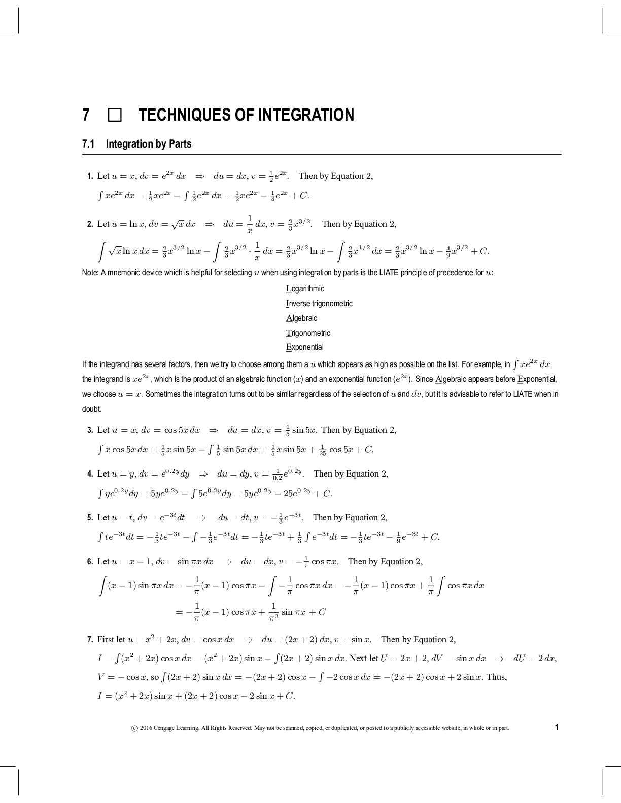
Buy this document to get the full access instantly
Instant Download Access after purchase
Add to cartInstant download
Reviews( 0 )
Document information
Connected school, study & course
About the document
Uploaded On
Jan 06, 2020
Number of pages
116
Written in

Additional information
This document has been written for:
Uploaded
Jan 06, 2020
Downloads
0
Views
63
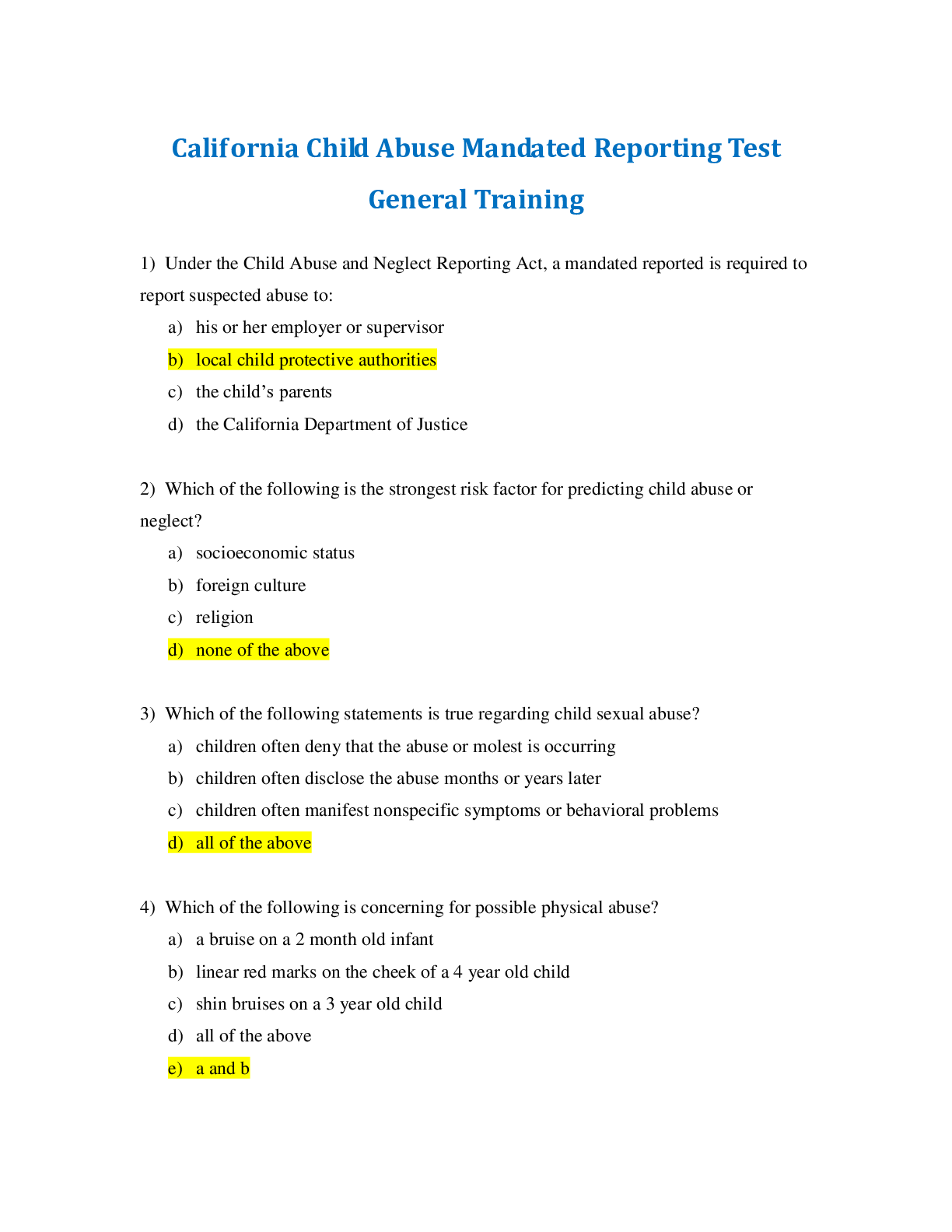
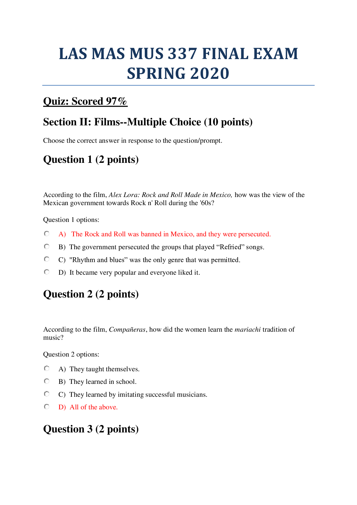
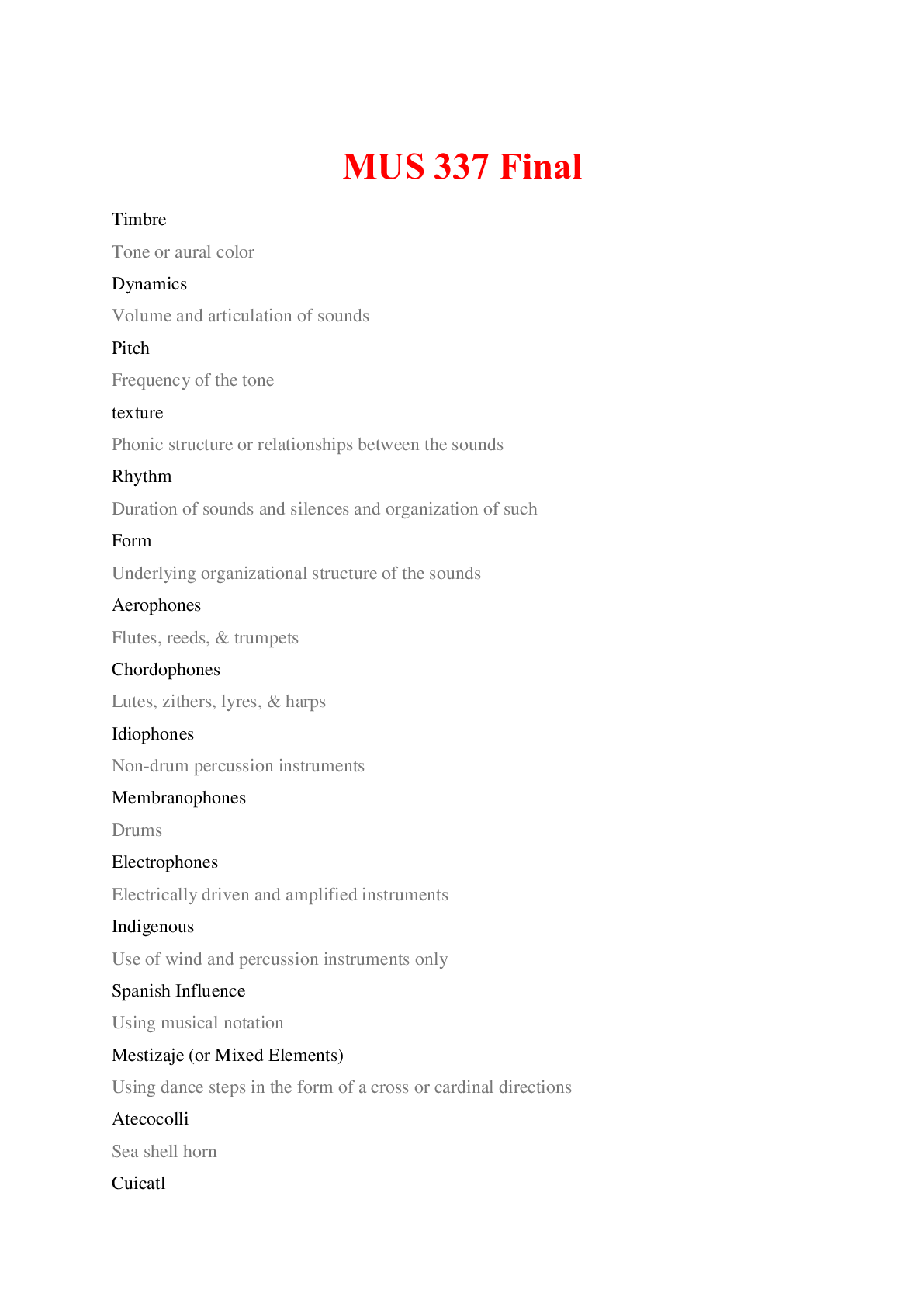
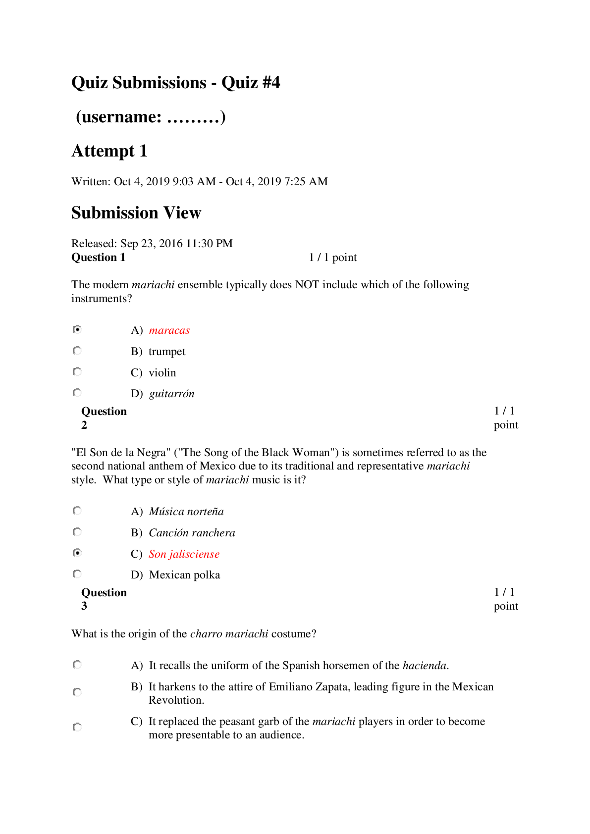

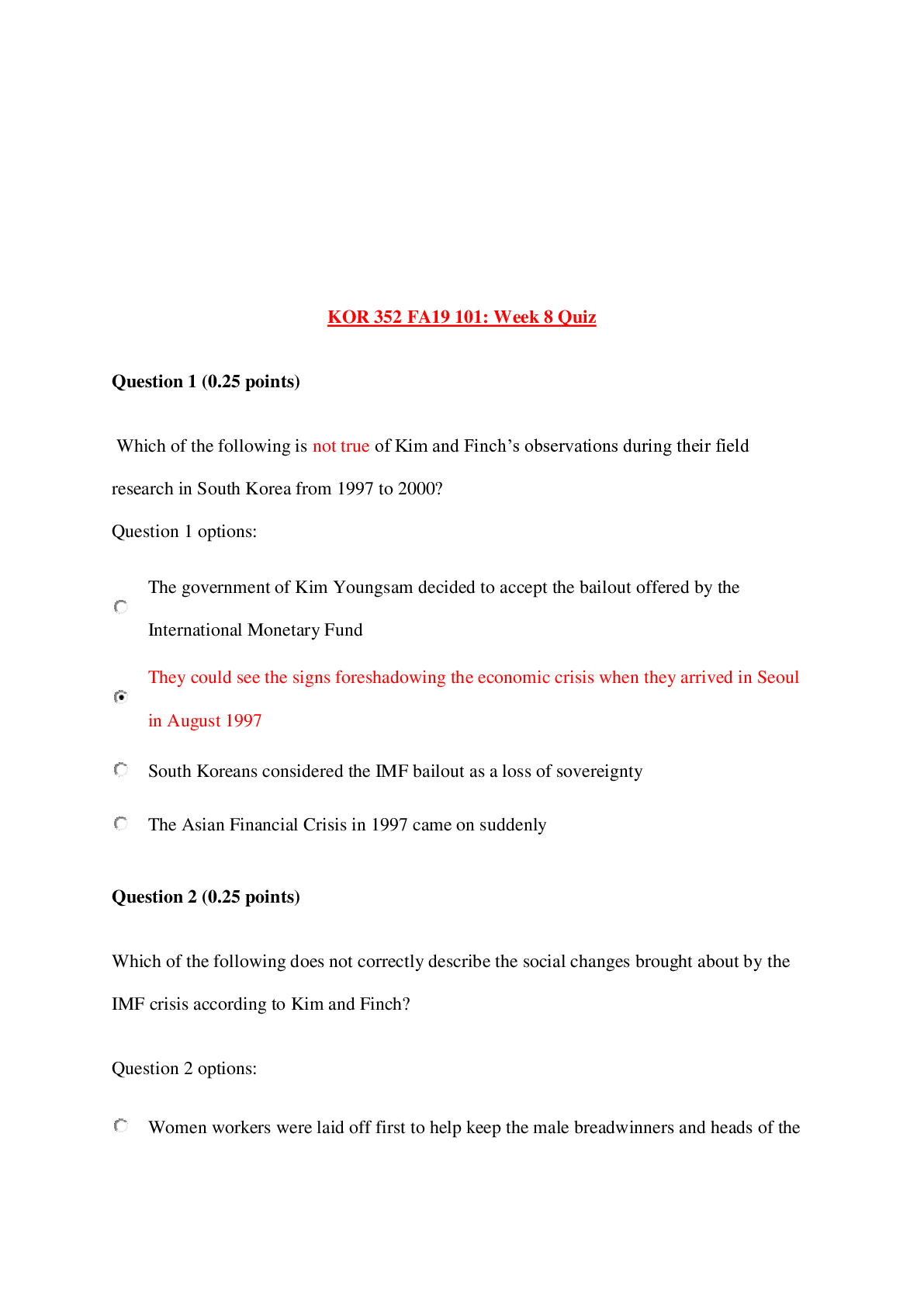


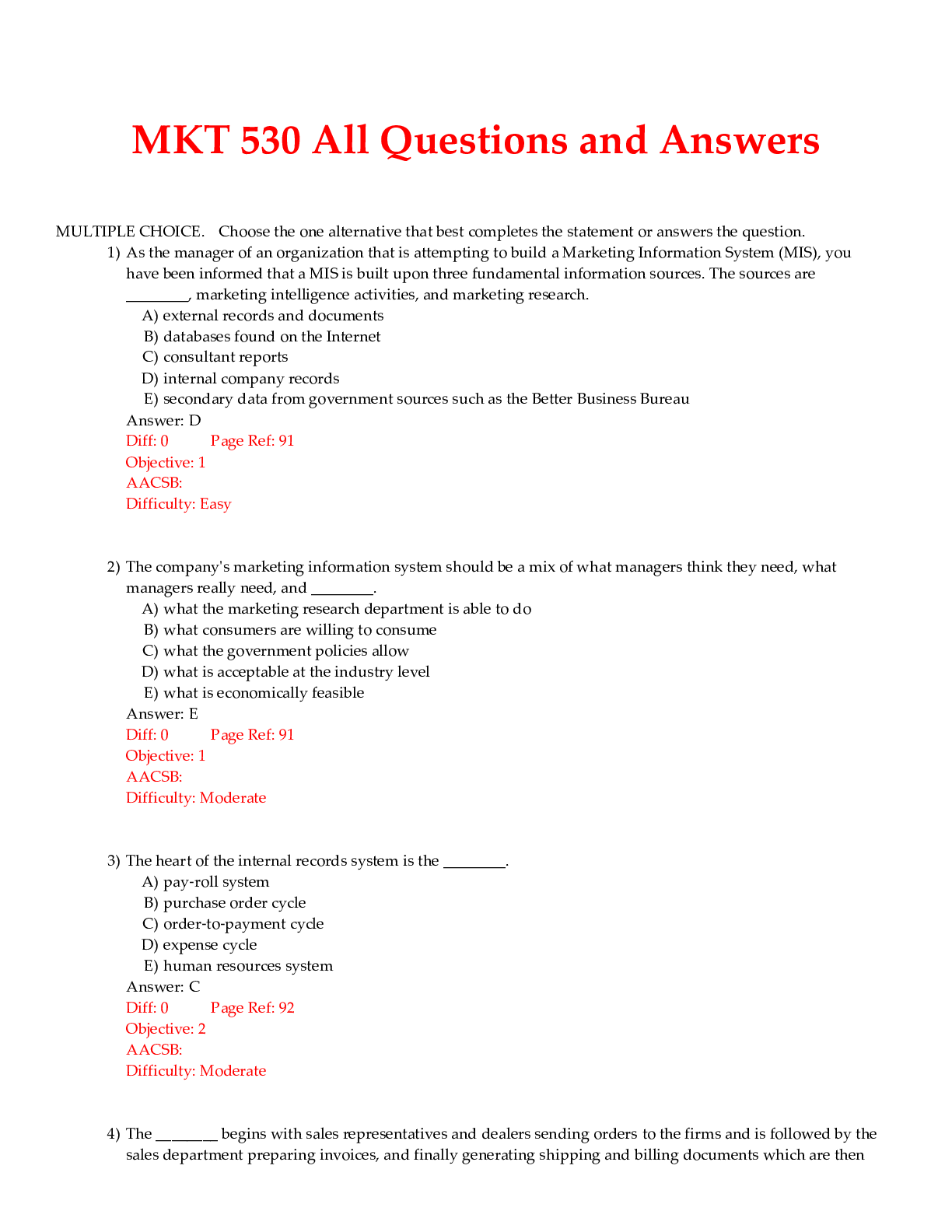


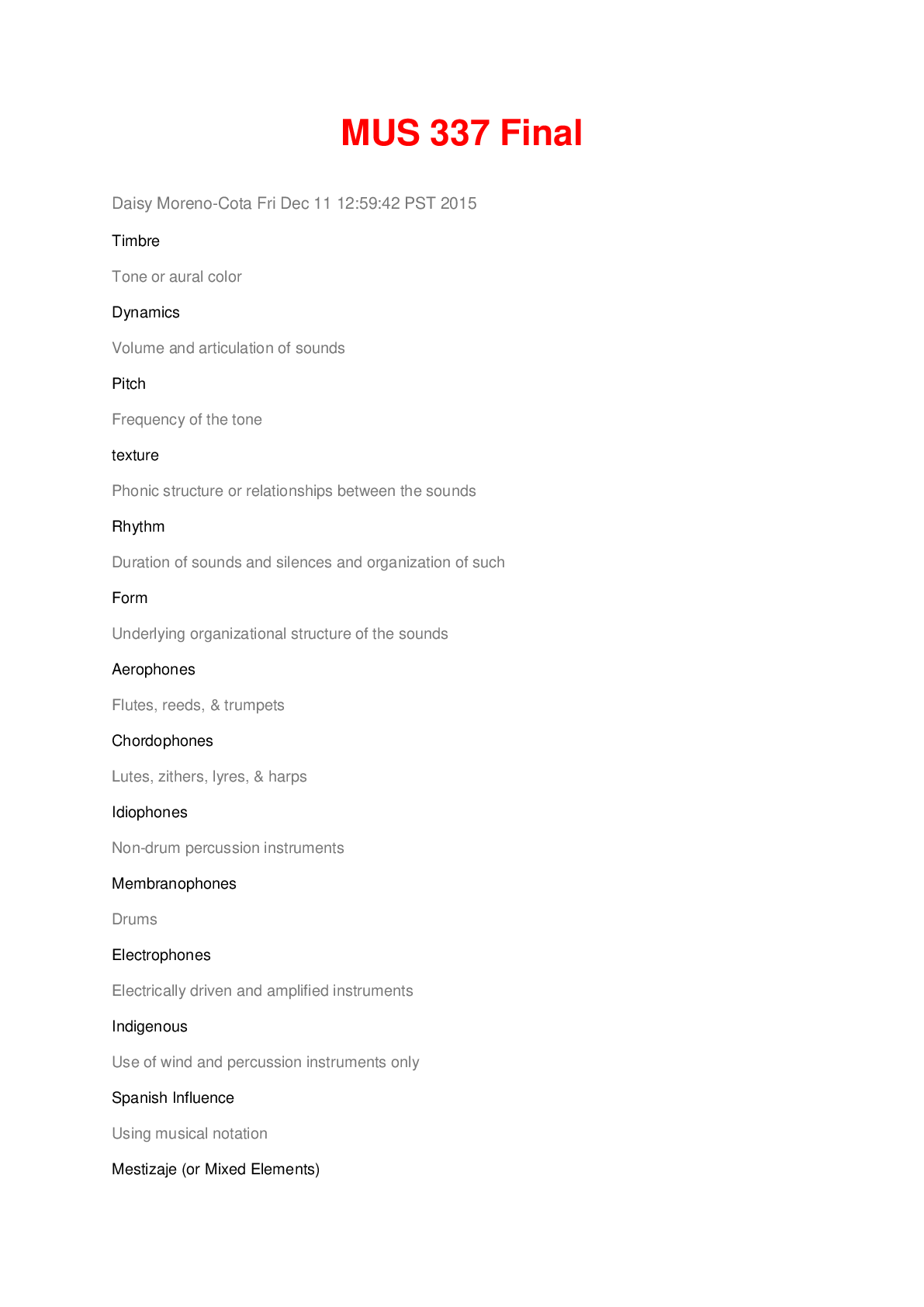
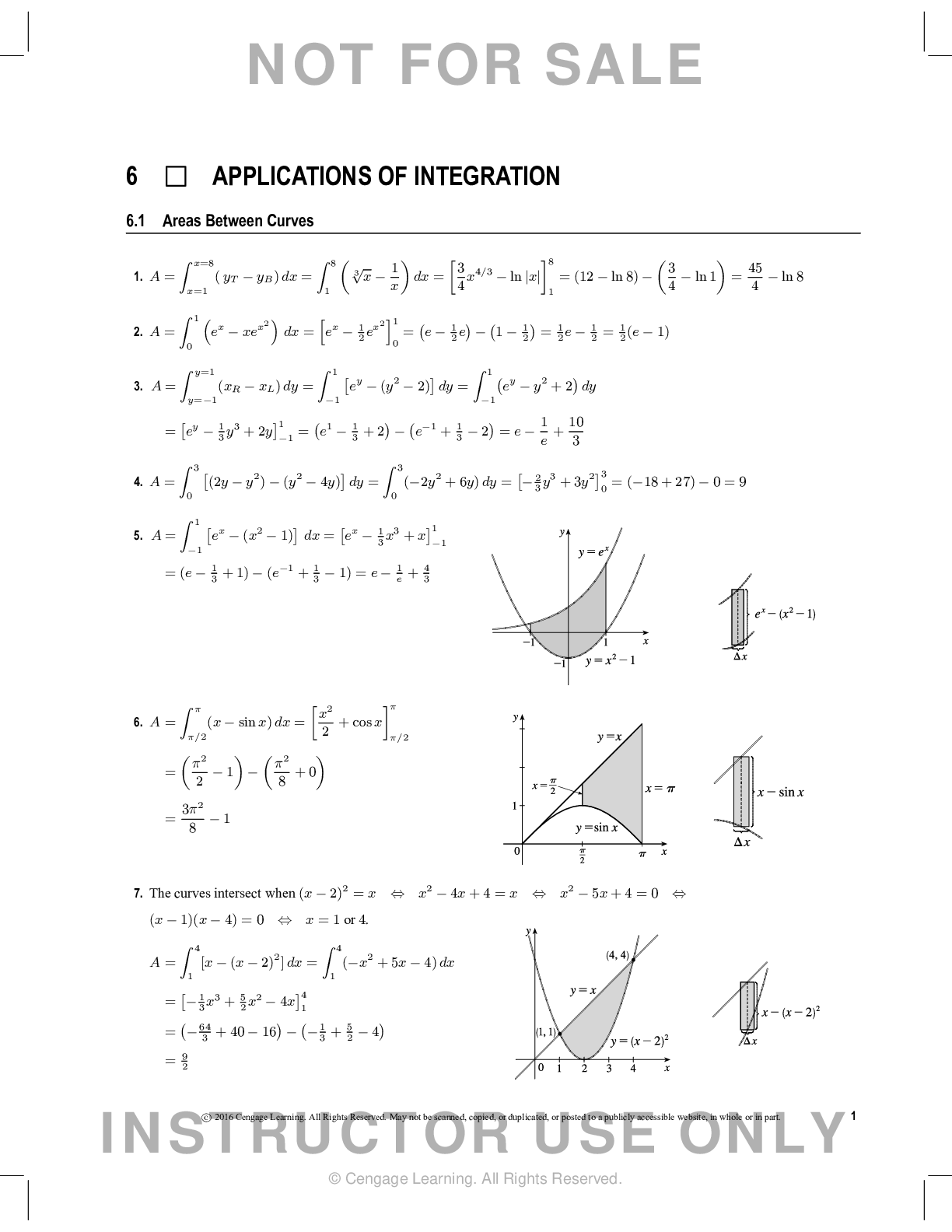

.png)
