Calculus > QUESTIONS & ANSWERS > Chapter 6: APPLICATIONS OF INTEGRATION. Work and Answers (All)
Chapter 6: APPLICATIONS OF INTEGRATION. Work and Answers
Document Content and Description Below
6.1 Areas Between Curves 1. = =1 =8( − ) = 18 √3 − 1 = 3 443 − ln||8 1 = (12 − ln 8) − 3 4 − ln 1 = 45 4 − l... n 8 2. = 01 − 2 = − 1 221 0 = − 1 2 − 1 − 1 2 = 1 2 − 1 2 = 1 2( − 1) 3. = ==1 −1( − ) = −11 − (2 − 2) = −11 − 2 + 2 = − 1 33 + 21 −1 = 1 − 1 3 + 2 − −1 + 1 3 − 2 = − 1 + 10 3 4. = 03 (2 − 2) − (2 − 4) = 03(−22 + 6) = − 2 33 + 323 0 = (−18 + 27) − 0 = 9 5. = −11 − (2 − 1) = − 1 33 + 1 −1 = ( − 1 3 + 1) − (−1 + 1 3 − 1) = − 1 + 4 3 6. = 2( − sin) = 22 + cos 2 = 22 − 1 − 82 + 0 = 32 8 − 1 7. The curves intersect when ( − 2)2 = ⇔ 2 − 4 + 4 = ⇔ 2 − 5 + 4 = 0 ⇔ ( − 1)( − 4) = 0 ⇔ = 1 or 4. = 14[ − ( − 2)2] = 14(−2 + 5 − 4) = − 1 33 + 5 22 − 44 1 = − 64 3 + 40 − 16 − − 1 3 + 5 2 − 4 = 9 2 °c 2016 Cengage Learning. All Rights Reserved. May not be scanned, copied, or duplicated, or posted to a publicly accessible website, in whole or in part. 1 NOT FOR SALE INSTRUCTOR USE ONLY © Cengage Learning. All Rights Reserved.2 ¤ CHAPTER 6 APPLICATIONS OF INTEGRATION 8. The curves intesect when 2 − 4 = 2 ⇒ 2 − 6 = 0 ⇒ ( − 6) = 0 ⇒ = 0 or 6. = 06[2 − (2 − 4)] = 06(6 − 2) = 32 − 1 336 0 = 3(6)2 − 1 3(6)3 − (0 − 0) = 108 − 72 = 36 9. = 12 1 − 12 = ln + 12 1 = ln 2 + 1 2 − (ln 1 + 1) = ln 2 − 1 2 ≈ 019 10. By observation, = sin and = 2 intersect at (00) and (21) for ≥ 0. = 02 sin − 2 = −cos − 1 2 0 2 = 0 − 4 − (−1) = 1 − 4 11. The curves intersect when 1 − 2 = 2 − 1 ⇔ 2 = 22 ⇔ 2 = 1 ⇔ = ±1. = −11 (1 − 2) − (2 − 1) = −11 2(1 − 2) = 2 · 201(1 − 2) = 4 − 1 331 0 = 41 − 1 3 = 8 3 12. 4 + 2 = 12 ⇔ ( + 6)( − 2) = 0 ⇔ = −6 or = 2, so = −6 or = 2 and = −26 − 1 42 + 3 − = − 12 1 3 − 1 22 + 32 −6 = − 2 3 − 2 + 6 − (18 − 18 − 18) = 22 − 2 3 = 64 3 °c 2016 Cengage Learning. All Rights Reserved. May not be scanned, copied, or duplicated, or posted to a publicly accessible website, in whole or in part. NOT FOR SALE INSTRUCTOR USE ONLY © Cengage Learning. All Rights Reserved.SECTION 6.1 AREAS BETWEEN CURVES ¤ 3 13. 12 − 2 = 2 − 6 ⇔ 22 = 18 ⇔ 2 = 9 ⇔ = ±3, so = −33 (12 − 2) − (2 − 6) = 203 18 − 22 [by symmetry] = 218 − 2 333 0 = 2 [(54 − 18) − 0] = 2(36) = 72 14. 2 = 4 − 2 ⇔ 22 − 4 = 0 ⇔ 2( − 2) = 0 ⇔ = 0 or 2, so = 02 (4 − 2) − 2 = 02(4 − 22) = 22 − 2 332 0 = 8 − 16 3 = 8 3 15. The curves intersect when 8cos = sec2 ⇒ 8cos3 = 1 ⇒ cos3 = 1 8 ⇒ cos = 1 2 ⇒ = 3 for 0 2 . By symmetry, = 203(8 cos − sec2 ) = 28sin − tan 0 3 = 28 · √23 − √3 = 23√3 = 6√3 16. = 02 [(2 − cos ) − cos] = 02(2 − 2cos) = 2 − 2sin2 0 = (4 − 0) − 0 = 4 17. 22 = 4 + 2 ⇔ 2 = 4 ⇔ = ±2, so = −22 (4 + 2) − 22 = 202(4 − 2) [by symmetry] = 24 − 1 332 0 = 28 − 8 3 = 32 3 °c 2016 Cengage Learning. All Rights Reserved. May not be scanned, copied, or duplicated, or posted to a publicly accessible website, in whole or in part. NOT FOR SALE INSTRUCTOR USE ONLY © Cengage Learning. All Rights Reserved.4 ¤ CHAPTER 6 APPLICATIONS OF INTEGRATION 18. The curves intersect when √ − 1 = − 1 ⇒ − 1 = 2 − 2 + 1 ⇔ 0 = 2 − 3 + 2 ⇔ 0 = ( − 1)( − 2) ⇔ = 1 or 2. = 12 √ − 1 − ( − 1) = 2 3( − 1)32 − 1 2( − 1)22 1 = 2 3 − 1 2 − (0 − 0) = 1 6 19. By inspection, the curves intersect at = ± 1 2. = −1122[cos − (42 − 1)] = 2012(cos − 42 + 1) [by symmetry] = 2 1 sin − 4 33 + 1 02 = 2 1 − 1 6 + 1 2 − 0 = 2 1 + 1 3 = 2 + 2 3 20. = √2 − ⇒ 2 = 2 − ⇔ = 2 − 2, so the curves intersect when 4 = 2 − 2 ⇔ 4 + 2 − 2 = 0 ⇔ (2 + 2)(2 − 1) = 0 ⇔ = 1 [since ≥ 0]. = 01[(2 − 2) − 4)] = 2 − 1 33 − 1 551 0 = 2 − 1 3 − 1 5 − 0 = 22 15 21. The curves intersect when tan = 2 sin (on [−3 3]) ⇔ sin = 2 sin cos ⇔ 2sin cos − sin = 0 ⇔ sin(2 cos − 1) = 0 ⇔ sin = 0 or cos = 1 2 ⇔ = 0 or = ± 3 . = 203(2 sin − tan) [by symmetry] = 2−2cos − ln|sec| 0 3 = 2 [(−1 − ln 2) − (−2 − 0)] = 2(1 − ln 2) = 2 − 2ln2 22. The curves intersect when 3 = ⇔ 3 − = 0 ⇔ (2 − 1) = 0 ⇔ ( + 1)( − 1) = 0 ⇔ = 0 or = ±1. = 201( − 3) [by symmetry] = 2 1 22 − 1 441 0 = 2 1 2 − 1 4 = 1 2 °c 2016 Cengage Learning. All Rights Reserved. May not be scanned, copied, or duplicated, or posted to a publicly accessible website, in whole or in part. NOT FOR SALE INSTRUCTOR USE ONLY © Cengage Learning. All Rights Reserved.SECTION 6.1 AREAS BETWEEN CURVES ¤ 5 23. The curves intersect when √3 2 = 1 82 ⇔ 2 = 1 (23)3 6 ⇔ 210 = 6 ⇔ 6 − 210 = 0 ⇔ (5 − 210) = 0 ⇔ = 0 or 5 = 210 ⇔ = 0 or = 22 = 4, so for 0 ≤ ≤ 6, = 04 √3 2 − 1 82 + 46 1 82 − √3 2 = 3 4 √3 243 − 24 1 34 0 + 24 1 3 − 3 4 √3 2436 4 = 3 4 √3 2 · 4√3 4 − 64 24 − (0 − 0) + 216 24 − 3 4 √3 2 · 6√3 6 − 64 24 − 3 4 √3 2 · 4√3 4 = 6 − 8 3 + 9 − 9 2 √3 12 − 8 3 + 6 = 47 3 − 9 2 √3 12 24. The curves intersect when cos = 1 − cos (on [0 ]) ⇔ 2cos = 1 ⇔ cos = 1 2 ⇔ = 3 . = 03 [cos − (1 − cos)] + 3 [(1 − cos ) − cos] = 03(2 cos − 1) + 3(1 − 2cos) = 2sin − 0 3 + − 2sin 3 = √3 − 3 − 0 + ( − 0) − 3 − √3 = 2√3 + 3 25. By inspection, we see that the curves intersect at = ±1 and that the area of the region enclosed by the curves is twice the area enclosed in the first quadrant. = 201 [(2 − ) − 4] = 22 − 1 22 − 1 551 0 = 22 − 1 2 − 1 5 − 0 = 2 13 10 = 13 5 °c 2016 Cengage Learning. All Rights Reserved. May not be scanned, copied, or duplicated, or posted to a publicly accessible website, in whole or in part. NOT FOR SALE INSTRUCTOR USE ONLY © Cengage Learning. All Rights Reserved.6 ¤ CHAPTER 6 APPLICATIONS OF INTEGRATION 26. sinh = − ⇔ 1 2( − −) = − ⇔ 1 2 = 3 2− ⇔ 2 = 3 ⇔ 2 = ln3 ⇔ = 1 2 ln3 (or ln√3). = 0ln √3(− − sinh) + ln2√3 (sinh − −) = −− − coshln 0 √3 + cosh + −2 ln √3 = −√13 − √23 − (−1 − 1) + (cosh 2 + −2) − √23 + √13 = −2√3 + 2 + cosh 2 + −2, or 2 − 2√3 + 1 22 + 3 2−2 27. 1 = ⇔ 1 = 2 ⇔ = ±1 and 1 = 1 4 ⇔ 4 = 2 ⇔ = ±2, so for 0, = 01 − 14 + 12 1 − 14 = 01 3 4 + 12 1 − 1 4 = 3 821 0 + ln|| − 1 822 1 = 3 8 + ln 2 − 1 2 − 0 − 1 8 = ln 2 28. 1 42 = − + 3 ⇔ 2 + 4 − 12 = 0 ⇔ ( + 6)( − 2) = 0 ⇔ = −6 or 2 and 22 = − + 3 ⇔ 22 + − 3 = 0 ⇔ (2 + 3)( − 1) = 0 ⇔ = − 3 2 or 1, so for ≥ 0, = 01 22 − 1 42 + 12 (− + 3) − 1 42 = 01 742 + 12 − 1 42 − + 3 = 12 7 31 0 + − 12 1 3 − 1 22 + 32 1 = 7 12 + − 2 3 − 2 + 6 − − 12 1 − 1 2 + 3 = 3 2 29. (a) Total area = 12 + 27 = 39. (b) () ≤ () for 0 ≤ ≤ 2 and () ≥ () for 2 ≤ ≤ 5, so 05[() − ()] = 02[() − ()] + 25[() − ()] = − 02[() − ()] + 25[() − ()] = −(12) + 27 = 15 30. √1 + 2 = √9− 2 ⇔ = 0 or √1 + 2 = √9 − 2 ⇒ 1 + 2 = 9 − 2 ⇒ 22 = 8 ⇒ 2 = 4 ⇒ = 2 ( ≥ 0). = 02 √1 + 2 − √9− 2 = 1 + 2 + 9 − 2 2 0 = (√5 + √5) − (1 + 3) = 2√5 − 4 °c 2016 Cengage Learning. All Rights Reserved. May not be scanned, copied, or duplicated, or posted to a publicly accessible website, in whole or in part. NOT FOR SALE INSTRUCTOR USE ONLY © Cengage Learning. All Rights Reserved.SECTION 6.1 AREAS BETWEEN CURVES ¤ 7 31. 1 + 2 = 2 1 + 3 ⇔ + 4 = 2 + 4 ⇔ = 2 ⇔ 0 = 2 − ⇔ 0 = ( − 1) ⇔ = 0 or = 1. = 01 1 +2 − 1 +23 = 1 2 ln(1 + 2) − 1 3 ln(1 + 3)1 0 = 1 2 ln 2 − 1 3 ln 2 − (0 − 0) = 1 6 ln 2 32. ln = (ln)2 ⇔ ln = (ln)2 ⇔ 0 = (ln)2 − ln ⇔ 0 = ln(ln − 1) ⇔ ln = 0 or 1 ⇔ = 0 or 1 [1 or ] = 1 ln − (ln)2 = 1 2(ln)2 − 1 3(ln)3 1 = 1 2 − 1 3 − (0 − 0) = 1 6 33. An equation of the line through (00) and (31) is = 1 3; through (0 0) and (1 2) is = 2; through (31) and (12) is = − 1 2 + 5 2 . = 01 2 − 1 3 + 13 − 1 2 + 5 2 − 1 3 = 01 5 3 + 13 − 5 6 + 5 2 = 5 621 0 + − 12 5 2 + 5 23 1 = 5 6 + − 15 4 + 15 2 − − 12 5 + 5 2 = 5 2 34. An equation of the line through (20) and (02) is = − + 2; through (20) and (−11) is = − 1 3 + 2 3 ; through (02) and (−11) is = + 2. = −01 ( + 2) − − 1 3 + 2 3 + 02 (− + 2) − − 1 3 + 2 3 = −01 4 3 + 4 3 + 02 − 2 3 + 4 3 = 2 32 + 4 30 −1 + − 1 32 + 4 32 0 = 0 − 2 3 − 4 3 + − 4 3 + 8 3 − 0 = 2 35. The curves intersect when sin = cos 2 (on [0 2]) ⇔ sin = 1 − 2sin2 ⇔ 2sin2 + sin − 1 = 0 ⇔ (2 sin − 1)(sin + 1) = 0 ⇒ sin = 1 2 ⇒ = 6 . = 02 |sin − cos 2| = 06(cos 2 − sin) + 62(sin − cos 2) = 1 2 sin 2 + cos 0 6 + −cos − 1 2 sin 2 2 6 = 1 4 √3 + 1 2 √3 − (0 + 1) + (0 − 0) − − 1 2 √3 − 1 4 √3 = 3 2 √3 − 1 °c 2016 Cengage Learning. All Rights Reserved. May not be scanned, copied, or duplicated, or posted to a publicly accessible website, in whole or in part. NOT FOR SALE INSTRUCTOR USE ONLY © Cengage Learning. All Rights Reserved.8 ¤ CHAPTER 6 APPLICATIONS OF INTEGRATION 36. = −11 |3 − 2| = −01(2 − 3) + 01(3 − 2) = ln 22 − ln 33 0 −1 + ln 3 3 − ln 2 2 1 0 = ln 2 1 − ln 3 1 − 2ln2 1 − 3ln3 1 + ln 3 3 − ln 2 2 − ln 3 1 − ln 2 1 = 2 − 1 − 4 + 2 2ln2 + −3 + 1 + 9 − 3 3ln3 = 4 3ln 3 − 1 2ln2 37. From the graph, we see that the curves intersect at = 0 and = ≈ 0896, with sin(2) 4 on (0 ). So the area of the region bounded by the curves is = 0 sin(2) − 4 = − 1 2 cos(2) − 1 55 0 = − 1 2 cos(2) − 1 55 + 1 2 ≈ 0037 38. From the graph, we see that the curves intersect (with ≥ 0) at = 0 and = , where ≈ 1052, with (2 + 1)2 5 − on (0 ). The area of the region bounded by the curves is = 0 (2 + 1) 2 − (5 − ) = −12 · 21+ 1 − 166 + 122 0 ≈ 059 39. From the graph, we see that the curves intersect at = ≈ −111 = ≈ 125 and = ≈ 286 with 3 − 3 + 4 32 − 2 on ( ) and 32 − 2 3 − 3 + 4 on ( ). So the area of the region bounded by the curves is = (3 − 3 + 4) − (32 − 2) + (32 − 2) − (3 − 3 + 4) = (3 − 32 − + 4) + (−3 + 32 + − 4) = 1 44 − 3 − 1 22 + 4 + − 1 44 + 3 + 1 22 − 4 ≈ 838 40. From the graph, we see that the curves intersect at = ≈ 029 and = ≈ 608. = 2√ is the upper curve, so the area of the region bounded by the curves is ≈ 2√ − 13 = 4 332 − ln 1 13 13 ≈ 511 °c 2016 Cengage Learning. All Rights Reserved. May not be scanned, copied, or duplicated, or posted to a publicly accessible website, in whole or in part. NOT FOR SALE INSTRUCTOR USE ONLY © Cengage Learning. All Rights Reserved.SECTION 6.1 AREAS BETWEEN CURVES ¤ 9 41. Graph Y1=2/(1+xˆ4) and Y2=xˆ2. We see that Y1 Y2 on (−1 1), so the area is given by −11 1 +24 − 2. Evaluate the integral with a command such as fnInt(Y1-Y2,x,-1,1) to get 280123 to five decimal places. Another method: Graph () = Y1=2/(1+xˆ4)-xˆ2 and from the graph evaluate () from −1 to 1. 42. The curves intersect at = ±1. = −11(1−2 − 4) ≈ 366016 43. The curves intersect at = 0 and = ≈ 0749363. = 0 √ − tan2 ≈ 025142 44. The curves intersect at = ≈ −1911917, = ≈ −1223676, and = ≈ 0607946. = ( + 2 sin4 ) − cos + cos − ( + 2 sin4 ) ≈ 170413 45. As the figure illustrates, the curves = and = 5 − 63 + 4 enclose a four-part region symmetric about the origin (since 5 − 63 + 4 and are odd functions of ). The curves intersect at values of where 5 − 63 + 4 = ; that is, where (4 − 62 + 3) = 0. That happens at = 0 and where 2 = 6 ± √36 − 12 2 = 3 ± √6; that is, at = −3 + √6, −3 − √6, 0, 3 − √6, and 3 + √6. The exact area is 2 √3+√6 0 (5 − 63 + 4) − = 2 √3+√6 0 5 − 63 + 3 = 2 √3−√6 0 (5 − 63 + 3) + 2 √3+√6 √3−√6 (−5 + 63 − 3) CAS = 12√6 − 9 °c 2016 Cengage Learning. All Rights Reserved. May not be scanned, copied, or duplicated, or posted to a publicly accessible website, in whole or in part. NOT FOR SALE INSTRUCTOR USE ONLY © Cengage Learning. All Rights Reserved.10 ¤ CHAPTER 6 APPLICATIONS OF INTEGRATION 46. The inequality ≥ 22 describes the region that lies on, or to the right of, the parabola = 22. The inequality ≤ 1 − || describes the region that lies on, or to the left of, the curve = 1 − || = 11 +− if if ≥ 0 0 . So the given region is the shaded region that lies between the curves. The graphs of = 1 − and = 22 intersect when 1 − = 22 ⇔ 22 + − 1 = 0 ⇔ (2 − 1)( + 1) = 0 ⇒ = 1 2 [for ≥ 0]. By symmetry, = 2012 (1 − ) − 22 = 2− 2 33 − 1 22 + 1 02 = 2− 12 1 − 1 8 + 1 2 − 0 = 2 24 7 = 12 7 . 47. 1 second = 1 3600 hour, so 10 s = 360 1 h. With the given data, we can take = 5 to use the Midpoint Rule. ∆ = 1360−0 5 = 1 1800, so distance Kelly − distance Chris = 01360 − 01360 = 01360 ( − ) ≈ 5 = 1 1800 [( − )(1) + ( − )(3) + ( − )(5) +( − )(7) + ( − )(9)] = 1 1800[(22 − 20) + (52 − 46) + (71 − 62) + (86 − 75) + (98 − 86)] = 1 1800(2 + 6 + 9 + 11 + 12) = 1800 1 (40) = 45 1 mile, or 117 1 3 feet 48. If = distance from left end of pool and = () = width at , then the Midpoint Rule with = 4 and ∆ = − = 8 · 2 − 0 4 = 4 gives Area = 016 ≈ 4(62 + 68 + 50 + 48) = 4(228) = 912 m2. 49. Let () denote the height of the wing at cm from the left end. ≈ 5 = 200 − 0 5 [(20) + (60) + (100) + (140) + (180)] = 40(203 + 290 + 273 + 205 + 87) = 40(1058) = 4232 cm2 50. For 0 ≤ ≤ 10, () (), so the area between the curves is given by 010 [() − ()] = 010(22000024 − 14600018) = 02200 0240024 − 01460 018001810 0 = 2753,000024 − 7309,000018 − 2753,000 − 7309,000 ≈ 8868 people This area A represents the increase in population over a 10-year period. 51. (a) From Example 5(a), the infectiousness concentration is 1210 cellsmL. () = 1210 ⇔ 09() = 1210 ⇔ 09(−)( − 21)( + 1) = 1210. Using a calculator to solve the last equation for 0 gives us two solutions with the lesser being = 3 ≈ 1126 days, or the 12th day. (b) From Example 5(b), the slope of the line through 1 and 2 is −23. From part (a), 3 = (3 1210). An equation of the line through 3 that is parallel to 12 is − 1210 = −23( − 3), or = −23 + 233 + 1210. Using a calculator, we °c 2016 Cengage Learning. All Rights Reserved. May not be scanned, copied, or duplicated, or posted to a publicly accessible website, in whole or in part. NOT FOR SALE INSTRUCTOR USE ONLY © Cengage Learning. All Rights Reserved.SECTION 6.1 AREAS BETWEEN CURVES ¤ 11 find that this line intersects at = 4 ≈ 1718, or the 18th day. So in the patient with some immunity, the infection lasts about 2 days less than in the patient without immunity. (c) The level of infectiousness for this patient is the area between the graph of and the line in part (b). This area is 34 () − (−23 + 233 + 1210) ≈ 1117 26 18(−093 + 182 + 419 − 146894) = −02254 + 63 + 20952 − 14689417 11 18 26 ≈ 706 52. From the figure, () () for 0 ≤ ≤ 2. The area between the curves is given by 02[() − ()] = 02[(0172 − 05 + 11) − (0733 − 22 + + 06)] = 02(−0733 + 2172 − 15 + 05) = −04734 + 2317 3 − 0752 + 052 0 = −292 + 1736 3 − 3 + 1 − 0 = 086 ≈ 087 Thus, about 0.87 more inches of rain fell at the second location than at the first during the first two hours of the storm. 53. We know that the area under curve between = 0 and = is 0 () = (), where () is the velocity of car A and A is its displacement. Similarly, the area under curve between = 0 and = is 0 B() = B(). (a) After one minute, the area under curve is greater than the area under curve . So car A is ahead after one minute. (b) The area of the shaded region has numerical value A(1) − B(1), which is the distance by which A is ahead of B after 1 minute. (c) After two minutes, car B is traveling faster than car A and has gained some ground, but the area under curve from = 0 to = 2 is still greater than the corresponding area for curve , so car A is still ahead. (d) From the graph, it appears that the area between curves and for 0 ≤ ≤ 1 (when car A is going faster), which corresponds to the distance by which car A is ahead, seems to be about 3 squares. Therefore, the cars will be side by side at the time where the area between the curves for 1 ≤ ≤ (when car B is going faster) is the same as the area for 0 ≤ ≤ 1. From the graph, it appears that this time is ≈ 22. So the cars are side by side when ≈ 22 minutes. 54. The area under 0() from = 50 to = 100 represents the change in revenue, and the area under 0() from = 50 to = 100 represents the change in cost. The shaded region represents the difference between these two values; that is, the increase in profit as the production level increases from 50 units to 100 units. We use the Midpoint Rule with = 5 and ∆ = 10: 5 = ∆{[0(55) − 0(55)] + [0(65) − 0(65)] + [0(75) − 0(75)] + [0(85) − 0(85)] + [0(95) − 0(95)]} ≈ 10(240 − 085 + 220 − 090 + 200 − 100 + 180 − 110 + 170 − 120) = 10(505) = 505 thousand dollars Using 1 would give us 50(2 − 1) = 50 thousand dollars. °c 2016 Cengage Learning. All Rights Reserved. May not be scanned, copied, or duplicated, or posted to a publicly accessible website, in whole or in part. NOT FOR SALE INSTRUCTOR USE ONLY © Cengage Learning. All Rights Reserved.12 ¤ CHAPTER 6 APPLICATIONS OF INTEGRATION 55. To graph this function, we must first express it as a combination of explicit functions of ; namely, = ± √ + 3. We can see from the graph that the loop extends from = −3 to = 0, and that by symmetry, the area we seek is just twice the area under the top half of the curve on this interval, the equation of the top half being = − √ + 3. So the area is = 2−03 − √ + 3 . We substitute = + 3, so = and the limits change to 0 and 3, and we get = −203 [( − 3)√] = −203(32 − 312) = −2 2 5 52 − 2323 0 = −2 2 5 32 √3 − 23√3 = 24 5 √3 56. We start by finding the equation of the tangent line to = 2 at the point (11): 0 = 2, so the slope of the tangent is 2(1) = 2, and its equation is − 1 = 2( − 1), or = 2 − 1. We would need two integrals to integrate with respect to , but only one to integrate with respect to . = 01 1 2( + 1) − √ = 1 4 2 + 1 2 − 2 3 321 0 = 1 4 + 1 2 − 2 3 = 1 12 57. By the symmetry of the problem, we consider only the first quadrant, where = 2 ⇒ = . We are looking for a number such that 0 = 4 ⇒ 2 3 32 0 = 2 3 324 ⇒ 32 = 432 − 32 ⇒ 232 = 8 ⇒ 32 = 4 ⇒ = 423 ≈ 252. 58. (a) We want to choose so that 1 12 = 4 12 ⇒ −1 1 = −14 ⇒ −1 + 1 = −1 4 + 1 ⇒ 5 4 = 2 ⇒ = 85. (b) The area under the curve = 12 from = 1 to = 4 is 3 4 [take = 4 in the first integral in part (a)]. Now the line = must intersect the curve = 1√ and not the line = 4, since the area under the line = 142 from = 1 to = 4 is only 16 3 , which is less than half of 3 4. We want to choose so that the upper area in the diagram is half of the total area under the curve = 12 from = 1 to = 4. This implies that 11√ − 1 = 1 2 · 3 4 ⇒ 2√ − 1 = 3 8 ⇒ 1 − 2√ + = 3 8 ⇒ − 2√ + 5 8 = 0. Letting = √, we get 2 − 2 + 5 8 = 0 ⇒ 82 − 16 + 5 = 0. Thus, = 16 ± √256 16 − 160 = 1 ± √46. But = √ 1 ⇒ = 1 − √6 4 ⇒ = 2 = 1 + 3 8 − √26 = 1 8 11 − 4√6 ≈ 01503. °c 2016 Cengage Learning. All Rights Reserved. May not be scanned, copied, or duplicated, or posted to a publicly accessible website, in whole or in part. NOT FOR SALE INSTRUCTOR USE ONLY © Cengage Learning. All Rights Reserved.SECTION 6.1 AREAS BETWEEN CURVES ¤ 13 59. We first assume that 0, since can be replaced by − in both equations without changing the graphs, and if = 0 the curves do not enclose a region. We see from the graph that the enclosed area lies between = − and = , and by symmetry, it is equal to four times the area in the first quadrant. The enclosed area is = 40 (2 − 2) = 42 − 1 3 3 0 = 43 − 1 3 3 = 4 2 3 3 = 8 3 3 So = 576 ⇔ 8 3 3 = 576 ⇔ 3 = 216 ⇔ = √3 216 = 6. Note that = −6 is another solution, since the graphs are the same. 60. It appears from the diagram that the curves = cos and = cos( − ) intersect halfway between 0 and , namely, when = 2. We can verify that this is indeed true by noting that cos(2 − ) = cos(−2) = cos(2). The point where cos( − ) crosses the -axis is = 2 + . So we require that 02 [cos − cos( − )] = − 2+ cos( − ) [the negative sign on the RHS is needed since the second area is beneath the -axis] ⇔ [sin − sin ( − )] 0 2 = −[sin ( − )] 2+ ⇒ [sin(2) − sin(−2)] − [−sin(−)] = −sin( − ) + sin 2 + − ⇔ 2sin(2) − sin = −sin + 1. [Here we have used the oddness of the sine function, and the fact that sin( − ) = sin]. So 2sin(2) = 1 ⇔ sin(2) = 1 2 ⇔ 2 = 6 ⇔ = 3 . 61. The curve and the line will determine a region when they intersect at two or more points. So we solve the equation (2 + 1) = ⇒ = (2 + ) ⇒ (2 + ) − = 0 ⇒ (2 + − 1) = 0 ⇒ = 0 or 2 + − 1 = 0 ⇒ = 0 or 2 = 1 − ⇒ = 0 or = ± 1 − 1. Note that if = 1, this has only the solution = 0, and no region is determined. But if 1 − 1 0 ⇔ 1 1 ⇔ 0 1, then there are two solutions. [Another way of seeing this is to observe that the slope of the tangent to = (2 + 1) at the origin is 0(0) = 1 and therefore we must have 0 1.] Note that we cannot just integrate between the positive and negative roots, since the curve and the line cross at the origin. Since and (2 + 1) are both odd functions, the total area is twice the area between the curves on the interval 0 1 − 1. So the total area enclosed is 20√1−1 2 + 1 − = 2 1 2 ln(2 + 1) − 1 2 2√ 0 1−1 = [ln(1 − 1 + 1) − (1 − 1)] − (ln 1 − 0) = ln(1) − 1 + = − ln − 1 °c 2016 Cengage Learning. All Rights Reserved. May not be scanned, copied, or duplicated, or posted to a publicly accessible website, in whole or in part. NOT FOR SALE INSTRUCTOR USE ONLY © Cengage Learning. All Rights Reserved.14 ¤ CHAPTER 6 APPLICATIONS OF INTEGRATION APPLIED PROJECT The Gini Index 1. (a) = area between and = area under = = 01 [ − ()] 1 2 = 201 [ − ()] (b) For a perfectly egalitarian society, () = , so = 201 [ − ] = 0. For a perfectly totalitarian society, () = 10 if if 0 ≤= 1 1 so = 201 ( − 0) = 2 1 221 0 = 2 1 2 = 1. 2. (a) The richest 20% of the population in 2010 received 1 − (08) = 1 − 0498 = 0502, or 502%, of the total US income. (b) A quadratic model has the form () = 2 + + . Rounding to six decimal places, we get = 1305 357, = −0371 357, and = 0026 714. The quadratic model appears to be a reasonable fit, but note that (0) 6= 0 and is both decreasing and increasing. (c) = 201[ − ()] ≈ 04477 3. () = 2 + + Year Gini 1970 1117 411 −0152 411 0013 321 03808 1980 1149 554 −0189 696 0016 179 03910 1990 1216 071 −0268 214 0020 714 04161 2000 1280 804 −0345 232 0025 821 04397 The Gini index has risen steadily from 1970 to 2010. The trend is toward a less egalitarian society. 4. Using Maple’s PowerFit or TI’s PwrReg command and omitting the point (00) gives us () = 08454462050 379 and a Gini index 201[ − ()] ≈ 04457. Note that the power function is nearly quadratic. 1 1.1 _0.1 _0.1 1.1 0.2 0.60.4 0.8 1 °c 2016 Cengage Learning. All Rights Reserved. May not be scanned, copied, or duplicated, or posted to a publicly accessible website, in whole or in part. NOT FOR SALE INSTRUCTOR USE ONLY © Cengage Learning. All Rights Reserved.SECTION 6.2 VOLUMES ¤ 15 6.2 Volumes 1. A cross-section is a disk with radius + 1, so its area is () = ( + 1)2 = (2 + 2 + 1). = 02 () = 02 (2 + 2 + 1) = 1 33 + 2 + 2 0 = 8 3 + 4 + 2 = 263 2. A cross-section is a disk with radius 1 , so its area is () = 12 = −2. = 14 () = 14 −2 = − −14 1 = − 1 4 + 1 = 3 4 3. A cross-section is a disk with radius √ − 1, so its area is () = √ − 12 = ( − 1). = 15 () = 15 ( − 1) = 1 22 − 5 1 = 25 2 − 5 − 1 2 − 1 = 8 4. A cross-section is a disk with radius , so its area is () = ()2 = 2 = −11 () = −11 2 = 1 221 −1 = 2 (2 − −2) °c 2016 Cengage Learning. All Rights Reserved. May not be scanned, copied, or duplicated, or posted to a publicly accessible website, in whole or in part. NOT FOR SALE INSTRUCTOR USE ONLY © Cengage Learning. All Rights Reserved.16 ¤ CHAPTER 6 APPLICATIONS OF INTEGRATION 5. A cross-section is a disk with radius 2, so its area is () = 2 2. = 09 () = 09 2 2 = 4 09 = 4 1 2 29 0 = 2(81) = 162 6. A cross-section is a disk with radius 1 22, so its area is () = 1 2 22 = 1 4 4. = 04 () = 04 1 44 = 4 1 5 54 0 = 20 (45) = 256 5 7. A cross-section is a washer (annulus) with inner radius 3 and outer radius , so its area is () = ()2 − (3)2 = (2 − 6). = 01 () = 01 (2 − 6) = 1 3 3 − 1 771 0 = 1 3 − 1 7 = 21 4 8. A cross-section is a washer (annulus) with inner radius 2 and outer radius 6 − 2, so its area is () = [(6 − 2)2 − 22] = (4 − 122 + 32). = −22 () = 202 (4 − 122 + 32) = 2 1 5 5 − 43 + 322 0 = 2 32 5 − 32 + 64 = 2 192 5 = 384 5 9. A cross-section is a washer with inner radius 2 and outer radius 2, so its area is () = (2)2 − (2)2 = (42 − 4). = 02 () = 02(42 − 4) = 4 3 3 − 1 552 0 = 32 3 − 32 5 = 64 15 °c 2016 Cengage Learning. All Rights Reserved. May not be scanned, copied, or duplicated, or posted to a publicly accessible website, in whole or in part. NOT FOR SALE INSTRUCTOR USE ONLY © Cengage Learning. All Rights Reserved.SECTION 6.2 VOLUMES ¤ 17 10. A cross-section is a washer with inner radius 4 and outer radius 2 − 2, so its area is () = (2−2)2 −(4)2 = (4−42 +4 −8). = −11 () = 201 (4 − 42 + 4 − 8) = 24 − 4 3 3 + 1 5 5 − 1 9 81 0 = 24 − 4 3 + 1 5 − 1 9 = 2 124 45 = 248 45 11. A cross-section is a washer with inner radius 1 − √ and outer radius 1 − 2, so its area is () = (1 − 2)2 − (1 − √)2 = (1 − 22 + 4) − (1 − 2√ + ) = 4 − 22 + 2√ − . = 01 () = 01 (4 − 22 + 212 − ) = 1 5 5 − 2 3 3 + 4 3 32 − 1 2 21 0 = 1 5 − 2 3 + 4 3 − 1 2 = 11 30 12. A cross-section is a washer with inner radius 1 − (−3) = 4 and outer radius 3 − (−3) = 3 + 3, so its area is () = (3 + 3)2 − (4)2 = (6 + 63 − 7). = 12 () = 12 (6 + 63 − 7) = 1 7 7 + 3 2 4 − 72 1 = 128 7 + 24 − 14 − 1 7 + 3 2 − 7 = 471 14 13. A cross-section is a washer with inner radius (1 + sec) − 1 = sec and outer radius 3 − 1 = 2, so its area is () = 22 − (sec)2 = (4 − sec2 ). = − 33 () = − 33 (4 − sec2 ) = 2 03(4 − sec2 ) [by symmetry] = 24 − tan 0 3 = 2 43 − √3 − 0 = 2 43 − √3 °c 2016 Cengage Learning. All Rights Reserved. May not be scanned, copied, or duplicated, or posted to a publicly accessible website, in whole or in part. NOT FOR SALE INSTRUCTOR USE ONLY © Cengage Learning. All Rights Reserved.18 ¤ CHAPTER 6 APPLICATIONS OF INTEGRATION 14. A cross-section is a washer with inner radius sin − (−1) and outer radius cos − (−1), so its area is () = (cos + 1)2 − (sin + 1)2 = (cos2 + 2cos − sin2 − 2sin) = (cos2 + 2cos − 2sin). = 04 () = 04 (cos 2 + 2 cos − 2sin) = 1 2 sin 2 + 2 sin + 2 cos 0 4 = 1 2 + √2 + √2 − (0 + 0 + 2) = 2√2 − 3 2 15. A cross-section is a washer with inner radius 2 − 1 and outer radius 2 − √3 , so its area is () = (2 − √3 )2 − (2 − 1)2 = 4 − 4√3 + 3 2 − 1. = 01 () = 01 (3 − 413 + 23) = 3 − 343 + 3 5231 0 = 3 − 3 + 3 5 = 3 5. 16. For 0 ≤ 1 2, a cross-section is a washer with inner radius 1 − (−1) and outer radius 2 − (−1), so its area is () = (32 − 22) = 5. For 1 2 ≤ ≤ 1, a cross-section is a washer with inner radius 1 − (−1) and outer radius 1 − (−1), so its area is () = (1 + 1)2 − (2)2 = (12 + 2 + 1 − 4). = 012 5 + 112 12 + 2 − 3 = 5 1 02 + −1 + 2 ln − 31 12 = 5 1 2 − 0 + (−1 + 0 − 3) − −2 + 2 ln 1 2 − 3 2 = 5 2 + − 1 2 + 2 ln 2 = (2 + 2 ln 2) = 2(1 + ln 2) °c 2016 Cengage Learning. All Rights Reserved. May not be scanned, copied, or duplicated, or posted to a publicly accessible website, in whole or in part. NOT FOR SALE INSTRUCTOR USE ONLY © Cengage Learning. All Rights Reserved.SECTION 6.2 VOLUMES ¤ 19 17. From the symmetry of the curves, we see they intersect at = 1 2 and so 2 = 1 2 ⇔ = ± 1 2. A cross-section is a washer with inner radius 3 − (1 − 2) and outer radius 3 − 2, so its area is () = (3 − 2)2 − (2 + 2)2 = (9 − 62 + 4) − (4 + 42 + 4) = (5 − 102). = −√√1122 () = 20√12 5(1 − 22) [by symmetry] = 10 − 2 33√ 0 22 = 10 √22 − √62 = 10 √32 = 10 3 √2 18. For 0 ≤ 2, a cross-section is an annulus with inner radius 2 − 1 and outer radius 4 − 1, the area of which is 1() = (4 − 1)2 − (2 − 1)2. For 2 ≤ ≤ 4, a cross-section is an annulus with inner radius − 1 and outer radius 4 − 1, the area of which is 2() = (4 − 1)2 − ( − 1)2. = 04 () = 02 (4 − 1)2 − (2 − 1)2 + 24 (4 − 1)2 − ( − 1)2 = 8 2 0 + 24(8 + 2 − 2) = 16 + 8 + 2 − 1 334 2 = 16 + 32 + 16 − 64 3 − 16 + 4 − 8 3 = 76 3 19. R1 about OA (the line = 0): = 01 () = 01 ()2 = 1 331 0 = 1 3 20. R1 about OC (the line = 0): = 01 () = 01 (12 − 2) = − 1 331 0 = 1 − 1 3 = 2 3 21. R1 about AB (the line = 1): = 01 () = 01 (1 − )2 = 01(1 − 2 + 2) = − 2 + 1 331 0 = 1 3 22. R1 about BC (the line = 1): = 01 () = 01 [(1 − 0)2 − (1 − )2] = 01[1 − (1 − 2 + 2)] = 01(−2 + 2) = − 1 33 + 21 0 = − 1 3 + 1 = 2 3 °c 2016 Cengage Learning. All Rights Reserved. May not be scanned, copied, or duplicated, or posted to a publicly accessible website, in whole or in part. NOT FOR SALE INSTRUCTOR USE ONLY © Cengage Learning. All Rights Reserved.20 ¤ CHAPTER 6 APPLICATIONS OF INTEGRATION 23. R2 about OA (the line = 0): = 01 () = 01 12 − √4 2 = 01(1 − 12) = − 2 3 321 0 = 1 − 2 3 = 1 3 24. R2 about OC (the line = 0): = 01 () = 01 [(4)2] = 01 8 = 1 9 91 0 = 1 9 25. R2 about AB (the line = 1): = 01 () = 01 [12 − (1 − 4)2] = 01[1 − (1 − 24 + 8)] = 01(24 − 8) = 2 5 5 − 1 9 91 0 = 2 5 − 1 9 = 13 45 26. R2 about BC (the line = 1): = 01 () = 01 (1 − √4 )2 = 01(1 − 214 + 12) = − 8 5 54 + 2 3 321 0 = 1 − 8 5 + 2 3 = 15 1 27. R3 about OA (the line = 0): = 01 () = 01 √4 2 − 2 = 01(12 − 2) = 2 3 32 − 1 331 0 = 2 3 − 1 3 = 1 3 Note: Let R = R1 ∪ R2 ∪ R3. If we rotate R about any of the segments , , , or , we obtain a right circular cylinder of height 1 and radius 1. Its volume is 2 = (1)2 · 1 = . As a check for Exercises 19, 23, and 27, we can add the answers, and that sum must equal . Thus, 1 3 + 1 3 + 1 3 = . 28. R3 about OC (the line = 0): = 01 () = 01 [2 − (4)2] = 01(2 − 8) = 1 33 − 1 9 91 0 = 1 3 − 1 9 = 2 9 Note: See the note in Exercise 27. For Exercises 20, 24, and 28, we have 2 3 + 1 9 + 2 9 = . 29. R3 about AB (the line = 1): = 01 () = 01 [(1 − 4)2 − (1 − )2] = 01[(1 − 24 + 8) − (1 − 2 + 2)] = 01(8 − 24 − 2 + 2) = 1 9 9 − 2 5 5 − 1 33 + 21 0 = 1 9 − 2 5 − 1 3 + 1 = 17 45 Note: See the note in Exercise 27. For Exercises 21, 25, and 29, we have 1 3 + 13 45 + 17 45 = . °c 2016 Cengage Learning. All Rights Reserved. May not be scanned, copied, or duplicated, or posted to a publicly accessible website, in whole or in part. NOT FOR SALE INSTRUCTOR USE ONLY © Cengage Learning. All Rights Reserved.SECTION 6.2 VOLUMES ¤ 21 30. R3 about BC (the line = 1): = 01 () = 01 [(1 − )2 − 1 − √4 2] = 01[(1 − 2 + 2) − (1 − 214 + 12)] = 01(2 − 2 − 12 + 214) = 1 3 3 − 2 − 2 3 32 + 8 5 541 0 = 1 3 − 1 − 2 3 + 8 5 = 15 4 Note: See the note in Exercise 27. For Exercises 22, 26, and 30, we have 2 3 + 15 1 + 15 4 = . 31. (a) About the -axis: = −11 (−2)2 = 2 01 −22 [by symmetry] ≈ 375825 (b) About = −1: = −11 [−2 − (−1)]2 − [0 − (−1)]2 = 2 01[(−2 + 1)2 − 1] = 2 01(−22 + 2−2) ≈ 1314312 32. (a) About the -axis: = − 22 (cos2 )2 = 2 02 cos4 [by symmetry] ≈ 370110 (b) About = 1: = − 22 [(1 − 0)2 − (1 − cos2 )2] = 2 02[1 − (1 − 2cos2 + cos4 )] = 2 02(2 cos2 − cos4 ) ≈ 616850 33. (a) About = 2: 2 + 42 = 4 ⇒ 42 = 4 − 2 ⇒ 2 = 1 − 24 ⇒ = ±1 − 24 = −22 2 − −1 − 242 − 2 − 1 − 242 = 2 02 81 − 24 ≈ 78.95684 °c 2016 Cengage Learning. All Rights Reserved. May not be scanned, copied, or duplicated, or posted to a publicly accessible website, in whole or in part. NOT FOR SALE INSTRUCTOR USE ONLY © Cengage Learning. All Rights Reserved.22 ¤ CHAPTER 6 APPLICATIONS OF INTEGRATION (b) About = 2: 2 + 42 = 4 ⇒ 2 = 4 − 42 ⇒ = ±4 − 42 = −11 2 − −4 − 42 2 − 2 − 4 − 42 2 = 2 01 84 − 42 ≈ 7895684 [Notice that this is the same approximation as in part (a). This can be explained by Pappus’s Theorem in Section 8.3.] 34. (a) About the -axis: = 2 and 2 + 2 = 1 ⇒ 2 + 4 = 1 ⇒ 4 + 2 − 1 = 0 ⇒ 2 = −1 + √5 2 ≈ 0618 ⇒ = ± = ±−1 +2 √5 ≈ ±0786. = − 1 − 2 2 − (2)2 = 2 0(1 − 2 − 4) ≈ 354459 (b) About the -axis: = 02 (√ )2 + 21 1 − 2 2 = 02 + 21(1 − 2) ≈ 099998 35. = ln(6 + 2) and = √3 − 3 intersect at = ≈ −4091, = ≈ −1467, and = ≈ 1091. = ln(6 + 2)2 − 3 − 3 2 + 3 − 3 2 − ln(6 + 2)2 ≈ 89023 36. = 1 + −3 and = arctan2 intersect at = ≈ −0570 and = ≈ 1391. = 1 + −32 − (arctan2)2 ≈ 6923 °c 2016 Cengage Learning. All Rights Reserved. May not be scanned, copied, or duplicated, or posted to a publicly accessible website, in whole or in part. NOT FOR SALE INSTRUCTOR USE ONLY © Cengage Learning. All Rights Reserved.SECTION 6.2 VOLUMES ¤ 23 37. = 0 sin2 − (−1)2 − [0 − (−1)]2 CAS = 11 8 2 38. = 02 (3 − )2 − (3 − 1−2)2 CAS = −22 + 24 − 142 3 39. 0 sin = 0 √sin 2 describes the volume of solid obtained by rotating the region R= ( ) | 0 ≤ ≤ , 0 ≤ ≤ √sin of the -plane about the -axis. 40. −11(1 − 2)2 describes the volume of the solid obtained by rotating the region R= {( ) | −1 ≤ ≤ 1, 0 ≤ ≤ 1 − 2} of the -plane about the -axis. 41. 01(4 − 8) = 01 (2)2 − (4)2 describes the volume of the solid obtained by rotating the region R = ( ) | 0 ≤ ≤ 1 4 ≤ ≤ 2 of the -plane about the -axis. 42. 14[32 − (3 − √)2 describes the volume of the solid obtained by rotating the region R = {( ) | 1 ≤ ≤ 43 − √ ≤ ≤ 3} of the -plane about the -axis. 43. There are 10 subintervals over the 15-cm length, so we’ll use = 102 = 5 for the Midpoint Rule. = 015 () ≈ 5 = 155−0[(15) + (45) + (75) + (105) + (135)] = 3(18 + 79 + 106 + 128 + 39) = 3 · 370 = 1110 cm3 44. = 010 () ≈ 5 = 105−0[(1) + (3) + (5) + (7) + (9)] = 2(065 + 061 + 059 + 055 + 050) = 2(290) = 580 m3 45. (a) = 210 [()]2 ≈ 104− 2 [(3)]2 + [(5)]2 + [(7)]2 + [(9)]2 ≈ 2 (15)2 + (22)2 + (38)2 + (31)2 ≈ 196 units3 (b) = 04 (outer radius)2 − (inner radius)2 ≈ 4 − 0 4 (99)2 − (22)2 + (97)2 − (30)2 + (93)2 − (56)2 + (87)2 − (65)2 ≈ 838 units3 °c 2016 Cengage Learning. All Rights Reserved. May not be scanned, copied, or duplicated, or posted to a publicly accessible website, in whole or in part. NOT FOR SALE INSTRUCTOR USE ONLY © Cengage Learning. All Rights Reserved.24 ¤ CHAPTER 6 APPLICATIONS OF INTEGRATION 46. (a) = −11 3 + 2 + + 1 − 2 2 CAS = 452 + 18 + 332315 + 14 + 7(2 + 52) (b) = (−0063 + 0042 + 01 + 054)√1 − 2 is graphed in the figure. Substitute = −006, = 004, = 01, and = 054 in the answer for part (a) to get CAS = 3769 9375 ≈ 1263. 47. We’ll form a right circular cone with height and base radius by revolving the line = about the -axis. = 0 2 = 0 22 2 = 22 1 33 0 = 2 2 1 33 = 132 Another solution: Revolve = − + about the -axis. = 0− + 2 =∗ 0 22 2 − 22 + 2 = 322 3 − 2 2 + 2 0 = 1 32 − 2 + 2 = 1 32 ∗ Or use substitution with = − and = − to get 0 2− = − 1 330 = − −133 = 132. 48. = 0 − − 2 = 0 2 − 2(− ) + − 2 2 = 2 − (− ) 2 + 1 3 − 23 0 = 2 − ( − ) + 1 3( − )2 = 1 3 3 + (2 − 2 + 2) = 1 3(2 + + 2) Another solution: = − by similar triangles. Therefore, = − ⇒ = ( − ) ⇒ °c 2016 Cengage Learning. All Rights Reserved. May not be scanned, copied, or duplicated, or posted to a publicly accessible website, in whole or in part. NOT FOR SALE INSTRUCTOR USE ONLY © Cengage Learning. All Rights Reserved.SECTION 6.2 VOLUMES ¤ 25 = − . Now = 1 32 − 1 32( − ) [by Exercise 47] = 1 3 2 − − 1 3 2 − − = = ( − ) = 1 3 3 − 3 − = 1 3 2 + + 2 = 1 3 2 + 2 + (2)(2) = 1 31 + 2 + √12 where 1 and 2 are the areas of the bases of the frustum. (See Exercise 50 for a related result.) 49. 2 + 2 = 2 ⇔ 2 = 2 − 2 = − 2 − 2 = 2 − 33 − = 3 − 33 − 2( − ) − ( −3)3 = 2 33 − 1 3( − )32 − ( − )2 = 1 3 23 − ( − )32 − 2 − 2 + 2 = 1 3 23 − ( − )22 + 2 − 2 = 1 3 23 − 23 − 22 + 2 + 22 + 22 − 3 = 1 3 32 − 3 = 1 32(3 − ), or, equivalently, 2 − 3 50. An equation of the line is = ∆ ∆ + (-intercept) = 2 −− 02 + 2 = 2− + 2 . = 0 () = 0(2)2 = 0 22− + 2 2 = 0 − + 2 = 0 ( −2)2 2 + 2(− ) + 2 = (3−2)2 3 + (− )2 + 2 0 = 1 3 ( − )2 + ( − ) + 2 = 1 32 − 2 + 2 + 3 = 1 3 2 + + 2 [Note that this can be written as 1 31 + 2 + √12 , as in Exercise 48.] If = , we get a rectangular solid with volume 2. If = 0, we get a square pyramid with volume 1 32. °c 2016 Cengage Learning. All Rights Reserved. May not be scanned, copied, or duplicated, or posted to a publicly accessible website, in whole or in part. NOT FOR SALE INSTRUCTOR USE ONLY © Cengage Learning. All Rights Reserved.26 ¤ CHAPTER 6 APPLICATIONS OF INTEGRATION 51. For a cross-section at height , we see from similar triangles that 2 2 = − , so = 1 − . Similarly, for cross-sections having 2 as their base and replacing , = 21 − . So = 0 () = 0 1 − 21 − = 0 221 − 2 = 22 01 − 2 + 22 = 22 − 2 + 332 0 = 22 − + 1 3 = 2 3 2 [ = 1 3 where is the area of the base, as with any pyramid.] 52. Consider the triangle consisting of two vertices of the base and the center of the base. This triangle is similar to the corresponding triangle at a height , so = ⇒ = . Also by similar triangles, = ( − ) ⇒ = ( − ). These two equations imply that = (1 − ), and since the cross-section is an equilateral triangle, it has area () = 1 2 · · √3 2 = 2(1 − )2 4 √3, so = 0 () = 24√3 01 − 2 = 2√3 4 −31 − 3 0 = −√1232(−1) = √1232 53. A cross-section at height is a triangle similar to the base, so we’ll multiply the legs of the base triangle, 3 and 4, by a proportionality factor of (5 − )5. Thus, the triangle at height has area () = 1 2 · 35 −5 · 45 −5 = 61 − 52, so = 05 () = 6051 − 52 = 610 2(−5) = 1 = −−1 5 5, = −30 1 330 1 = −30− 1 3 = 10 cm3 54. A cross-section is shaded in the diagram. () = (2)2 = 2√2 − 2 2, so = − () = 20 4(2 − 2) = 82 − 1 3 3 0 = 8 2 3 3 = 16 3 3 °c 2016 Cengage Learning. All Rights Reserved. May not be scanned, copied, or duplicated, or posted to a publicly accessible website, in whole or in part. NOT FOR SALE INSTRUCTOR USE ONLY © Cengage Learning. All Rights Reserved.SECTION 6.2 VOLUMES ¤ 27 55. If is a leg of the isosceles right triangle and 2 is the hypotenuse, then 2 + 2 = (2)2 ⇒ 22 = 42 ⇒ 2 = 22. = −22 () = 202 () = 202 12()() = 202 2 = 202 1 4(36 − 92) = 9 2 02(4 − 2) = 9 2 4 − 1 332 0 = 9 2 8 − 8 3 = 24 56. The cross-section of the base corresponding to the coordinate has length = 1 − The corresponding equilateral triangle with side has area () = 2 √43 = (1 − )2 √43 Therefore, = 01 () = 01 (1 − )2 √43 = √3 4 01(1 − 2 + 2) = √43 − 2 + 1 331 0 = √3 4 31 = √123 Or: 01 (1 − )2 √43 = √43 10 2(−) [ = 1 − ] = √43 1331 0 = √123 57. The cross-section of the base corresponding to the coordinate has length = 1 − . The corresponding square with side has area () = 2 = (1 − )2 = 1 − 2 + 2. Therefore, = 01 () = 01(1 − 2 + 2) = − 2 + 1 331 0 = 1 − 1 + 1 3 − 0 = 1 3 Or: 01(1 − )2 = 10 2(−) [ = 1 − ] = 1 331 0 = 1 3 58. The cross-section of the base corresponding to the coordinate has length 2 = 2√1 − . = 1 − 2 ⇔ = ±√1 − The corresponding square with side has area () = 2 = 2√1 − 2 = 4(1 − ). Therefore, = 01 () = 01 4(1 − ) = 4 − 1 221 0 = 41 − 1 2 − 0 = 2. 59. The cross-section of the base corresponding to the coordinate has length 1 − 2. The height also has length 1 − 2, so the corresponding isosceles triangle has area () = 1 2 = 1 2(1 − 2)2. Therefore, = −11 () = −11 1 2(1 − 2)2 = 2 · 1 2 01(1 − 22 + 4) [by symmetry] = − 2 33 + 1 551 0 = 1 − 2 3 + 1 5 − 0 = 15 8 °c 2016 Cengage Learning. All Rights Reserved. May not be scanned, copied, or duplicated, or posted to a publicly accessible website, in whole or in part. NOT FOR SALE INSTRUCTOR USE ONLY © Cengage Learning. All Rights Reserved.28 ¤ CHAPTER 6 APPLICATIONS OF INTEGRATION 60. The cross-section of the base corresponding to the coordinate has length 2 = 2√2 − . [ = 2 − 2 ⇔ = ±√2 − ] The corresponding cross-section of the solid is a quarter-circle with radius 2√2 − and area () = 1 4 (2√2 − )2 = (2 − ). Therefore, = 02 () = 02 (2 − ) = 2 − 1 2 22 0 = (4 − 2) = 2 61. The cross-section of at coordinate , −1 ≤ ≤ 1, is a circle centered at the point 1 2(1 − 2) with radius 1 2(1 − 2). The area of the cross-section is () = 1 2(1 − 2)2 = 4 (1 − 22 + 4) The volume of is = −11 () = 201 4(1 − 22 + 4) = 2 − 2 3 3 + 1 551 0 = 2 1 − 2 3 + 1 5 = 2 15 8 = 415 62. (a) = − () = 20 () = 20 1 2 2√2 − 2 = 2 0 √2 − 2 (b) Observe that the integral represents one quarter of the area of a circle of radius , so = 2 · 1 42 = 1 2 2. 63. (a) The torus is obtained by rotating the circle ( − )2 + 2 = 2 about the -axis. Solving for , we see that the right half of the circle is given by = + 2 − 2 = () and the left half by = − 2 − 2 = (). So = − [()]2 − [()]2 = 2 0 2 + 2 2 − 2 + 2 − 2 − 2 − 2 2 − 2 + 2 − 2 = 2 0 4 2 − 2 = 8 0 2 − 2 (b) Observe that the integral represents a quarter of the area of a circle with radius , so 8 0 2 − 2 = 8 · 1 4 2 = 222. 64. The cross-sections perpendicular to the -axis in Figure 17 are rectangles. The rectangle corresponding to the coordinate has a base of length 216 − 2 in the -plane and a height of √13 , since ∠ = 30◦ and || = √13 ||. Thus, () = √23 16 − 2 and = 04 () = √23 04 16 − 2 = √23 16 0 12− 1 2 [Put = 16 − 2, so = −2 ] = 1√ 3 016 12 = √13 233216 0 = 3√2 3 (64) = 3128 √3 °c 2016 Cengage Learning. All Rights Reserved. May not be scanned, copied, or duplicated, or posted to a publicly accessible website, in whole or in part. NOT FOR SALE INSTRUCTOR USE ONLY © Cengage Learning. All Rights Reserved.SECTION 6.2 VOLUMES ¤ 29 65. (a) Volume(1) = 0 () = Volume(2) since the cross-sectional area () at height is the same for both solids. (b) By Cavalieri’s Principle, the volume of the cylinder in the figure is the same as that of a right circular cylinder with radius and height , that is, 2. 66. Each cross-section of the solid in a plane perpendicular to the -axis is a square (since the edges of the cut lie on the cylinders, which are perpendicular). One-quarter of this square and one-eighth of are shown. The area of this quarter-square is ||2 = 2 − 2. Therefore, () = 4(2 − 2) and the volume of is = − () = 4−(2 − 2) = 8(2 − 2) = 82 − 1 33 0 = 16 3 3 67. The volume is obtained by rotating the area common to two circles of radius , as shown. The volume of the right half is right = 02 2 = 02 2 − 1 2 + 2 = 2 − 1 3 1 2 + 3 0 2 = 1 23 − 1 33 − 0 − 24 1 3 = 24 5 3 So by symmetry, the total volume is twice this, or 12 5 3. Another solution: We observe that the volume is the twice the volume of a cap of a sphere, so we can use the formula from Exercise 49 with = 1 2: = 2 · 1 32(3 − ) = 2 3 1 223 − 1 2 = 12 5 3. 68. We consider two cases: one in which the ball is not completely submerged and the other in which it is. Case 1: 0 ≤ ≤ 10 The ball will not be completely submerged, and so a cross-section of the water parallel to the surface will be the shaded area shown in the first diagram. We can find the area of the cross-section at height above the bottom of the bowl by using the Pythagorean Theorem: 2 = 152 − (15 − )2 and 2 = 52 − ( − 5)2, so () = 2 − 2 = 20. The volume of water when it has depth is then () = 0 () = 0 20 = 102 0 = 102 cm3, 0 ≤ ≤ 10. Case 2: 10 ≤ 15 In this case we can find the volume by simply subtracting the volume displaced by the ball from the total volume inside the bowl underneath the surface of the water. The total volume underneath the surface is just the volume of a cap of the bowl, so we use the formula from Exercise 49: cap() = 1 32(45 − ). The volume of the small sphere is ball = 4 3(5)3 = 500 3 , so the total volume is cap − ball = 1 3(452 − 3 − 500) cm3. °c 2016 Cengage Learning. All Rights Reserved. May not be scanned, copied, or duplicated, or posted to a publicly accessible website, in whole or in part. NOT FOR SALE INSTRUCTOR USE ONLY © Cengage Learning. All Rights Reserved.30 ¤ CHAPTER 6 APPLICATIONS OF INTEGRATION 69. Take the -axis to be the axis of the cylindrical hole of radius . A quarter of the cross-section through perpendicular to the -axis, is the rectangle shown. Using the Pythagorean Theorem twice, we see that the dimensions of this rectangle are = 2 − 2 and = 2 − 2, so 1 4 () = = 2 − 2 2 − 2, and = − () = − 42 − 2 2 − 2 = 80 2 − 2 2 − 2 70. The line = intersects the semicircle = √2 − 2 when = √2 − 2 ⇒ 2 = 2 − 2 ⇒ 2 = 2 − 2 ⇒ = ±√2 − 2. Rotating the shaded region about the -axis gives us = −√√22−−22 2 − 2 2 − 2 = 2 0√2−2(2 − 2 − 2) [by symmetry] = 2 0√2−2 2 − 2 − 2 = 22 − 2 − 1 33√ 0 2−2 = 22 − 232 − 1 32 − 232 = 2 · 2 32 − 232 = 43 2 − 232 Our answer makes sense in limiting cases. As → 0, → 4 33, which is the volume of the full sphere. As → , → 0, which makes sense because the hole’s radius is approaching that of the sphere. 71. (a) The radius of the barrel is the same at each end by symmetry, since the function = − 2 is even. Since the barrel is obtained by rotating the graph of the function about the -axis, this radius is equal to the value of at = 1 2, which is − 1 22 = − = . (b) The barrel is symmetric about the -axis, so its volume is twice the volume of that part of the barrel for 0. Also, the barrel is a volume of rotation, so = 202 2 = 2 02 − 22 = 22 − 2 33 + 1 525 0 2 = 2 1 22 − 12 1 3 + 160 1 25 [continued] °c 2016 Cengage Learning. All Rights Reserved. May not be scanned, copied, or duplicated, or posted to a publicly accessible website, in whole or in part. NOT FOR SALE INSTRUCTOR USE ONLY © Cengage Learning. All Rights Reserved.SECTION 6.3 VOLUMES BY CYLINDRICAL SHELLS ¤ 31 Trying to make this look more like the expression we want, we rewrite it as = 1 322 + 2 − 1 22 + 80 3 24. But 2 − 1 22 + 80 3 24 = − 1 422 − 40 1 24 = ( − )2 − 2 5 1 422 = 2 − 2 52. Substituting this back into , we see that = 1 322 + 2 − 2 5 2, as required. 72. It suffices to consider the case where R is bounded by the curves = () and = () for ≤ ≤ , where () ≤ () for all in [ ], since other regions can be decomposed into subregions of this type. We are concerned with the volume obtained when R is rotated about the line = −, which is equal to 2 = [() + ]2 − [() + ]2 = [()]2 − [()]2 + 2 [() − ()] = 1 + 2 6.3 Volumes by Cylindrical Shells 1. If we were to use the “washer” method, we would first have to locate the local maximum point ( ) of = ( − 1)2 using the methods of Chapter 4. Then we would have to solve the equation = ( − 1)2 for in terms of to obtain the functions = 1() and = 2() shown in the first figure. This step would be difficult because it involves the cubic formula. Finally we would find the volume using = 0 [1()]2 − [2()]2 . Using shells, we find that a typical approximating shell has radius , so its circumference is 2. Its height is , that is, ( − 1)2. So the total volume is = 01 2( − 1)2 = 2 01 4 − 23 + 2 = 255 − 244 + 33 1 0 = 15 2. A typical cylindrical shell has circumference 2 and height sin(2). = 0√ 2sin(2). Let = 2. Then = 2 , so = 0 sin = [−cos] 0 = [1 − (−1)] = 2. For slicing, we would first have to locate the local maximum point ( ) of = sin(2) using the methods of Chapter 4. Then we would have to solve the equation = sin2 for in terms of to obtain the functions = 1() and = 2() shown in the second figure. Finally we would find the volume using = 0 [1()]2 − [2()]2 . Using shells is definitely preferable to slicing. °c 2016 Cengage Learning. All Rights Reserved. May not be scanned, copied, or duplicated, or posted to a publicly accessible website, in whole or in part. NOT FOR SALE INSTRUCTOR USE ONLY © Cengage Learning. All Rights Reserved.32 ¤ CHAPTER 6 APPLICATIONS OF INTEGRATION 3. = 01 2√3 = 2 01 43 = 2 3 7731 0 = 2 3 7 = 6 7 4. = 12 2 · 3 = 2 12 4 = 2 1 552 1 = 2 32 5 − 1 5 = 62 5 5. = 01 2−2 . Let = 2. Thus, = 2 , so = 01 − = −−1 0 = (1 − 1). 6. 4 − 2 = ⇔ 0 = 2 − 3 ⇔ 0 = ( − 3) ⇔ = 0 or 3. = 03 2[(4 − 2) − ] = 2 03(−3 + 32) = 2− 1 44 + 33 0 = 2− 81 4 + 27 = 2 27 4 = 27 2 7. 2 = 6 − 22 ⇔ 32 − 6 = 0 ⇔ 3( − 2) = 0 ⇔ = 0 or 2. = 02 2[(6 − 22) − 2] = 2 02(−33 + 62) = 2− 3 44 + 232 0 = 2 (−12 + 16) = 8 °c 2016 Cengage Learning. All Rights Reserved. May not be scanned, copied, or duplicated, or posted to a publicly accessible website, in whole or in part. NOT FOR SALE INSTRUCTOR USE ONLY © Cengage Learning. All Rights Reserved.SECTION 6.3 VOLUMES BY CYLINDRICAL SHELLS ¤ 33 8. By slicing: = 01 2 − (2)2 = 01( − 4) = 1 22 − 1 551 0 = 1 2 − 1 5 = 10 3 By cylindrical shells: = 01 2√ − 2 = 2 01(32 − 3) = 2 2 552 − 1 441 0 = 2 2 5 − 1 4 = 2 20 3 = 10 3 9. = 1 ⇒ = 1 . The shell has radius , circumference 2, and height 1, so = 13 21 = 2 13 = 23 1 = 2(3 − 1) = 4 10. = √ ⇒ = 2. The shell has radius , circumference 2, and height 2, so = 02 2(2) = 2 02 3 = 2 1 442 0 = 2(4) = 8 11. = 32 ⇒ = 23. The shell has radius , circumference 2, and height 23, so = 08 2(23) = 2 08 53 = 2 3 8838 0 = 2 · 3 8 · 256 = 192 °c 2016 Cengage Learning. All Rights Reserved. May not be scanned, copied, or duplicated, or posted to a publicly accessible website, in whole or in part. NOT FOR SALE INSTRUCTOR USE ONLY © Cengage Learning. All Rights Reserved.34 ¤ CHAPTER 6 APPLICATIONS OF INTEGRATION 12. The shell has radius , circumference 2, and height −32 + 12 − 9, so = 13 2(−32 + 12 − 9) = 2 13(−33 + 122 − 9) = −6 13(3 − 42 + 3) = −6 1 44 − 4 3 3 + 3 2 23 1 = −6 81 4 − 36 + 27 2 − 1 4 − 4 3 + 3 2 = −6− 8 3 = 16 13. The shell has radius , circumference 2, and height 2 − 1 + ( − 2)2 = 1 − ( − 2)2 = 1 − 2 − 4 + 4 = −2 + 4 − 3, so = 13 2(−2 + 4 − 3) = 2 13(−3 + 42 − 3) = 2− 1 4 4 + 4 3 3 − 3 2 23 1 = 2− 81 4 + 36 − 27 2 − − 1 4 + 4 3 − 3 2 = 2 8 3 = 16 3 14. The curves intersect when 4 − = 2 − 4 + 4 ⇔ 0 = 2 − 3 ⇔ 0 = ( − 3) ⇔ = 0 or 3. The shell has radius , circumference 2, and height (4 − ) − (2 − 4 + 4) = −2 + 3, so = 03 2(−2 + 3) = 2 03(32 − 3) = 23 − 1 443 0 = 227 − 81 4 = 2 27 4 = 272 15. The shell has radius 3 − , circumference 2(3 − ), and height 8 − 3. = 02 2(3 − )(8 − 3) = 2 02(4 − 33 − 8 + 24) = 2 1 5 5 − 3 4 4 − 42 + 242 0 = 2 32 5 − 12 − 16 + 48 = 2 132 5 = 264 5 °c 2016 Cengage Learning. All Rights Reserved. May not be scanned, copied, or duplicated, or posted to a publicly accessible website, in whole or in part. NOT FOR SALE INSTRUCTOR USE ONLY © Cengage Learning. All Rights Reserved.SECTION 6.3 VOLUMES BY CYLINDRICAL SHELLS ¤ 35 16. The shell has radius − (−1) = + 1, circumference 2( + 1), and height 4 − 2. = 02 2( + 1)(4 − 2) = 4 02( + 1)(2 − ) = 4 02(−2 + + 2) = 4 − 1 33 + 1 22 + 22 0 = 4 − 8 3 + 2 + 4 = 4 10 3 = 403 17. The shell has radius − 1, circumference 2( − 1), and height (4 − 2) − 3 = −2 + 4 − 3. = 13 2( − 1)(−2 + 4 − 3) = 2 13(−3 + 52 − 7 + 3) = 2− 1 44 + 5 33 − 7 22 + 33 1 = 2− 81 4 + 45 − 63 2 + 9 − − 1 4 + 5 3 − 7 2 + 3 = 2 4 3 = 8 3 18. The shell has radius 5 − , circumference 2(5 − ), and height √ − 1 2. = 04 2(5 − )√ − 1 2 = 2 04(512 − 5 2 − 32 + 1 22) = 2 10 3 32 − 5 42 − 2 552 + 1 634 0 = 2 80 3 − 20 − 64 5 + 32 3 = 2 68 15 = 136 15 19. The shell has radius 2 − , circumference 2(2 − ), and height 2 − 22. = 01 2(2 − )(2 − 22) = 4 01(2 − )(1 − 2) = 4 01(3 − 22 − + 2) = 4 1 44 − 2 33 − 1 22 + 21 0 = 4 1 4 − 2 3 − 1 2 + 2 = 4 13 12 = 133 °c 2016 Cengage Learning. All Rights Reserved. May not be scanned, copied, or duplicated, or posted to a publicly accessible website, in whole or in part. NOT FOR SALE INSTRUCTOR USE ONLY © Cengage Learning. All Rights Reserved.36 ¤ CHAPTER 6 APPLICATIONS OF INTEGRATION 20. The shell has radius − (−2) = + 2, circumference 2( + 2), and height (2 + 1) − 22 = 1 − 2. = −11 2( + 2)(1 − 2) = 2 −11(−3 − 22 + + 2) = 4 01(−22 + 2) [by Theorem 5.5.7] = 8 01(1 − 2) = 8 − 1 3 31 0 = 81 − 1 3 = 8 2 3 = 163 21. (a) = 2 02 (−) = 2 02 2− (b) ≈ 406300 22. (a) = 2 04 2 − tan (b) ≈ 225323 23. (a) = 2 − 22( − )[cos4 − (−cos4 )] = 4 − 22( − ) cos4 [or 82 02 cos4 using Theorem 5.5.7] (b) ≈ 4650942 24. (a) = 2 1 + 3 ⇒ + 4 = 2 ⇒ 4 − = 0 ⇒ (3 − 1) = 0 ⇒ ( − 1)(2 + + 1) = 0 ⇒ = 0 or 1 = 2 01[ − (−1)] 1 +23 − (b) ≈ 236164 °c 2016 Cengage Learning. All Rights Reserved. May not be scanned, copied, or duplicated, or posted to a publicly accessible website, in whole or in part. NOT FOR SALE INSTRUCTOR USE ONLY © Cengage Learning. All Rights Reserved.SECTION 6.3 VOLUMES BY CYLINDRICAL SHELLS ¤ 37 25. (a) = 0 2(4 − )√sin (b) ≈ 3657476 26. (a) = −33 2(5 − )4 − 2 + 7 (b) ≈ 16302712 27. = 01 2√1 + 3 . Let () = √1 + 3. Then the Midpoint Rule with = 5 gives 01 () ≈ 1−5 0 [(01) + (03) + (05) + (07) + (09)] ≈ 02(29290) Multiplying by 2 gives ≈ 368. 28. = 010 2(). Let () = (), where the values of are obtained from the graph. Using the Midpoint Rule with = 5 gives 010 () ≈ 105−0[(1) + (3) + (5) + (7) + (9)] = 2[1(1) + 3(3) + 5(5) + 7(7) + 9(9)] = 2[1(4 − 2) + 3(5 − 1) + 5(4 − 1) + 7(4 − 2) + 9(4 − 2)] = 2(2 + 12 + 15 + 14 + 18) = 2(61) = 122 Multiplying by 2 gives ≈ 244 ≈ 7665. 29. 03 25 = 2 03 (4). The solid is obtained by rotating the region 0 ≤ ≤ 4, 0 ≤ ≤ 3 about the y-axis using cylindrical shells. 30. 13 2 ln . The solid is obtained by rotating the region 0 ≤ ≤ ln, 1 ≤ ≤ 3 about the -axis using cylindrical shells. °c 2016 Cengage Learning. All Rights Reserved. May not be scanned, copied, or duplicated, or posted to a publicly accessible website, in whole or in part. NOT FOR SALE INSTRUCTOR USE ONLY © Cengage Learning. All Rights Reserved.38 ¤ CHAPTER 6 APPLICATIONS OF INTEGRATION 31. 2 14 + 2 2 = 2 14( + 2)12 . The solid is obtained by rotating the region 0 ≤ ≤ 12, 1 ≤ ≤ 4 about the line = −2 using cylindrical shells. 32. 01 2(2 − )(3 − 2). The solid is obtained by rotating the region 2 ≤ ≤ 3, 0 ≤ ≤ 1 about the line = 2 using cylindrical shells. 33. From the graph, the curves intersect at = 0 and = ≈ 2175, with 2 + 1 2 − 2 on the interval (0 ). So the volume of the solid obtained by rotating the region about the -axis is = 2 0 2+ 1 − (2 − 2) ≈ 14450 34. From the graph, the curves intersect at = ≈ 0906 and = ≈ 2715, with sin 2 − 4 + 5 on the interval ( ). So the volume of the solid obtained by rotating the region about the -axis is = 2 sin − (2 − 4 + 5) ≈ 21253 35. = 2 02 2 − sin2 − sin4 CAS = 1 323 36. = 2 0 [ − (−1)](3 sin) CAS = 2(4 + 3 − 122 − 6 + 48) = 25 + 24 − 243 − 122 + 96 37. Use shells: = 24 2(−2 + 6 − 8) = 2 24(−3 + 62 − 8) = 2 − 1 44 + 23 − 424 2 = 2[(−64 + 128 − 64) − (−4 + 16 − 16)] = 2(4) = 8 °c 2016 Cengage Learning. All Rights Reserved. May not be scanned, copied, or duplicated, or posted to a publicly accessible website, in whole or in part. NOT FOR SALE INSTRUCTOR USE ONLY © Cengage Learning. All Rights Reserved.SECTION 6.3 VOLUMES BY CYLINDRICAL SHELLS ¤ 39 38. Use disks: = 24 (−2 + 6 − 8)2 = 24(4 − 123 + 522 − 96 + 64) = 1 55 − 34 + 52 3 3 − 482 + 644 2 = 512 15 − 496 15 = 16 15 39. Use washers: 2 − 2 = 1 ⇒ = ±√2 ± 1 = −√√33 (2 − 0)2 − 2 + 1 − 02 = 2 0√3[4 − (2 + 1)] [by symmetry] = 2 0√3(3 − 2) = 2 3 − 1 33√ 0 3 = 23√3 − √3 = 4√3 40. Use disks: 2 − 2 = 1 ⇒ = ±2 − 1 = 12 2 − 12 = 12(2 − 1) = 1 33 − 2 1 = 8 3 − 2 − 1 3 − 1 = 4 3 41. Use disks: 2 + ( − 1)2 = 1 ⇔ = ±1 − ( − 1)2 = 02 1 − ( − 1)2 2 = 02 (2 − 2) = 2 − 1 332 0 = 4 − 8 3 = 4 3 42. Use shells: = 15 2( − 1)[4 − ( − 3)2] = 2 15( − 1)(−2 + 6 − 5) = 2 15(−3 + 72 − 11 + 5) = 2− 1 44 + 7 33 − 11 2 2 + 55 1 = 2 275 12 − 19 12 = 128 3 °c 2016 Cengage Learning. All Rights Reserved. May not be scanned, copied, or duplicated, or posted to a publicly accessible website, in whole or in part. NOT FOR SALE INSTRUCTOR USE ONLY © Cengage Learning. All Rights Reserved.40 ¤ CHAPTER 6 APPLICATIONS OF INTEGRATION 43. + 1 = ( − 1)2 ⇔ + 1 = 2 − 2 + 1 ⇔ 0 = 2 − 3 ⇔ 0 = ( − 3) ⇔ = 0 or 3. Use disks: = 03 [( + 1) − (−1)]2 − [( − 1)2 − (−1)]2 = 03[( + 2)2 − (2 − 2 + 2)2] = 03[(2 + 4 + 4) − (4 − 43 + 82 − 8 + 4)] = 03(−4 + 43 − 72 + 12) = − 1 5 5 + 4 − 7 3 3 + 623 0 = − 243 5 + 81 − 63 + 54 = 117 5 44. Use cylindrical shells to find the volume . = 01 2( − )(2) = 4 01( − 2) = 4 1 2 2 − 1 331 0 = 4 1 2 − 1 3 Now solve for in terms of : = 4 1 2 − 1 3 ⇔ 4 = 12 − 13 ⇔ 12 = 4 + 13 ⇔ = 2 + 2 3 45. Use shells: = 20 2√2 − 2 = −2 0(2 − 2)12(−2) = −2 · 2 3(2 − 2)32 0 = − 4 3 (0 − 3) = 4 3 3 46. = −+ 2 · 22 − ( − )2 = − 4( + )√2 − 2 [let = − ] = 4 − √2 − 2 + 4 − √2 − 2 The first integral is the area of a semicircle of radius , that is, 1 2 2, and the second is zero since the integrand is an odd function. Thus, = 4 1 2 2 + 4 · 0 = 222. 47. = 2 0 − + = 2 0 −2 + = 2−33 + 22 0 = 2 62 = 32 °c 2016 Cengage Learning. All Rights Reserved. May not be scanned, copied, or duplicated, or posted to a publicly accessible website, in whole or in part. NOT FOR SALE INSTRUCTOR USE ONLY © Cengage Learning. All Rights Reserved.SECTION 6.4 WORK ¤ 41 48. By symmetry, the volume of a napkin ring obtained by drilling a hole of radius through a sphere with radius is twice the volume obtained by rotating the area above the -axis and below the curve = √2 − 2 (the equation of the top half of the cross-section of the sphere), between = and = , about the -axis. This volume is equal to 2inner radius outer radius 2 = 2 · 2 2 − 2 = 4− 1 3 2 − 232 = 4 3 (2 − 2)32 But by the Pythagorean Theorem, 2 − 2 = 1 2 2, so the volume of the napkin ring is 4 3 1 2 3 = 1 6 3, which is independent of both and ; that is, the amount of wood in a napkin ring of height is the same regardless of the size of the sphere used. Note that most of this calculation has been done already, but with more difficulty, in Exercise 6.2.70. Another solution: The height of the missing cap is the radius of the sphere minus half the height of the cut-out cylinder, that is, − 1 2 . Using Exercise 6.2.49, napkin ring = sphere − cylinder − 2cap = 4 3 3 − 2 − 2 · 3 − 1 2 23 − − 1 2 = 1 6 3 6.4 Work 1. (a) The work done by the gorilla in lifting its weight of 360 pounds to a height of 20 feet is = = (360 lb)(20 ft) = 7200 ft-lb. (b) The amount of time it takes the gorilla to climb the tree doesn’t change the amount of work done, so the work done is still 7200 ft-lb. 2. = = () = [(200 kg)(98 ms2)](3 m) = (1960 N)(3 m) = 5880 J 3. = () = 110 5−2 = 5−−110 1 = 5− 10 1 + 1 = 45 ft-lb 4. = 12 cos 1 3 = 3 sin 1 3 2 1 = 3 √23 − √23 = 0 N·m = 0 J. Interpretation: From = 1 to = 3 2, the force does work equal to 132 cos 1 3 = 3 1 − √23 J in accelerating the particle and increasing its kinetic energy. From = 3 2 to = 2, the force opposes the motion of the particle, decreasing its kinetic energy. This is negative work, equal in magnitude but opposite in sign to the work done from = 1 to = 3 2. 5. The force function is given by () (in newtons) and the work (in joules) is the area under the curve, given by 08 () = 04 () + 48 () = 1 2(4)(30) + (4)(30) = 180 J. 6. = 420 () ≈ 4 = ∆[(6) + (10) + (14) + (18)] = 204−4[58 + 88 + 82 + 52] = 4(28) = 112 J 7. According to Hooke’s Law, the force required to maintain a spring stretched units beyond its natural length (or compressed units less than its natural length) is proportional to , that is, () = . Here, the amount stretched is 4in. = 1 3 ft and °c 2016 Cengage Learning. All Rights Reserved. May not be scanned, copied, or duplicated, or posted to a publicly accessible website, in whole or in part. NOT FOR SALE INSTRUCTOR USE ONLY © Cengage Learning. All Rights Reserved.42 ¤ CHAPTER 6 APPLICATIONS OF INTEGRATION the force is 10 lb. Thus, 10 = 1 3 ⇒ = 30 lbft, and () = 30. The work done in stretching the spring from its natural length to 6in. = 1 2 ft beyond its natural length is = 012 30 = 1521 02 = 15 4 ft-lb. 8. According to Hooke’s Law, the force required to maintain a spring stretched units beyond its natural length (or compressed units less than its natural length) is proportional to , that is, () = . Here, the amount compressed is 40 − 30 = 10 cm = 01 m and the force is 60 N. Thus, 60 = (01) ⇒ = 600 Nm, and () = 600. The work required to compress the spring 01 m is = 001 600 = 30020 01 = 300(001) = 3 N-m (or J). The work required to compress the spring 40 − 25 = 15 cm = 015 m is = 0015 600 = 30020 015 = 300(00225) = 675 J. 9. (a) If 0012 = 2 J, then 2 = 1 220 012 = 1 2(00144) = 00072 and = 00072 2 = 2500 9 ≈ 27778 Nm. Thus, the work needed to stretch the spring from 35 cm to 40 cm is 0005 10 2500 9 = 1250 9 21 1 10 20 = 1250 9 100 1 − 400 1 = 25 24 ≈ 104 J. (b) () = , so 30 = 2500 9 and = 2500 270 m = 108 cm 10. If 12 = 01 = 1 221 0 = 1 2, then = 24 lbft and the work required is 034 24 = 1223 04 = 12 · 16 9 = 27 4 = 675 ft-lb. 11. The distance from 20 cm to 30 cm is 01 m, so with () = , we get 1 = 001 = 1 220 01 = 200 1 . Now 2 = 0012 = 1 220 0 2 1 = 200 4 − 200 1 = 200 3 . Thus, 2 = 31. 12. Let be the natural length of the spring in meters. Then 6 = 0010 12−− = 1 220 0 12 10− − = 1 2(012 − )2 − (010 − )2 and 10 = 0012 14−− = 1 220 0 14 12− − = 1 2(014 − )2 − (012 − )2. Simplifying gives us 12 = (00044 − 004) and 20 = (00052 − 004). Subtracting the first equation from the second gives 8 = 00008, so = 10,000. Now the second equation becomes 20 = 52 − 400, so = 400 32 m = 8 cm. In Exercises 13 – 22, is the number of subintervals of length ∆, and ∗ is a sample point in the th subinterval [−1 ]. 13. (a) The portion of the rope from ft to ( + ∆) ft below the top of the building weighs 1 2 ∆ lb and must be lifted ∗ ft, so its contribution to the total work is 1 2∗ ∆ ft-lb. The total work is = lim →∞ =1 1 2 ∗ ∆ = 050 1 2 = 1 4250 0 = 2500 4 = 625 ft-lb Notice that the exact height of the building does not matter (as long as it is more than 50 ft). (b) When half the rope is pulled to the top of the building, the work to lift the top half of the rope is 1 = 025 1 2 = 1 4225 0 = 625 4 ft-lb. The bottom half of the rope is lifted 25 ft and the work needed to accomplish °c 2016 Cengage Learning. All Rights Reserved. May not be scanned, copied, or duplicated, or posted to a publicly accessible website, in whole or in part. NOT FOR SALE INSTRUCTOR USE ONLY © Cengage Learning. All Rights Reserved.SECTION 6.4 WORK ¤ 43 that is 2 = 25 50 1 2 · 25 = 25 2 50 25 = 625 2 ft-lb. The total work done in pulling half the rope to the top of the building is = 1 + 2 = 625 2 + 625 4 = 3 4 · 625 = 1875 4 ft-lb. 14. (a) The 60 ft cable weighs 180 lb, or 3 lbft. If we divide the cable into equal parts of length ∆ = 60 ft, then for large , all points in the th part are lifted by approximately the same amount. Choose a representative distance from the winch in the th part of the cable, say ∗ . If ∗ 25 ft, then the th part has to be lifted roughly ∗ ft. If ∗ ≥ 25 ft, then the th part has to be lifted 25 ft. The th part weighs (3 lbft)(∆ ft) = 3∆ lb, so the work done in lifting it is (3∆)∗ if ∗ 25 ft and (3∆)(25) = 75∆ if ∗ ≥ 25 ft. The work of lifting the top 25 ft of the cable is 1 = lim →∞ 1 =1 3∗ ∆ = 025 3 = 3 2225 0 = 3 2(625) = 9375 ft-lb. Here 1 represents the number of parts of the cable in the top 25 ft. The work of lifting the bottom 35 ft of the cable is 2 = lim →∞ 2 =1 75∆ = 25 60 75 = 75(60 − 25) = 2625 ft-lb, where 2 represents the number of small parts in the bottom 35 feet of the cable. The total work done is = 1 + 2 = 9375 + 2625 = 35625 ft-lb. (b) Once feet of cable have been wound up by the winch, there is (60 − ) ft of cable still hanging from the winch. That portion of the cable weighs 3(60 − ) lb. Lifting it ∆ feet requires 3(60 − )∆ ft-lb of work. Thus, the total work needed to lift the cable 25 ft is = 025 3(60 − ) = 180 − 3 2225 0 = 4500 − 9375 = 35625 ft-lb. 15. The work needed to lift the cable is lim →∞ =1 2∗ ∆ = 0500 2 = 2500 0 = 250,000 ft-lb. The work needed to lift the coal is 800 lb · 500 ft = 400,000 ft-lb. Thus, the total work required is 250,000 + 400,000 = 650,000 ft-lb. 16. Assumptions: 1. After lifting, the chain is L-shaped, with 4 m of the chain lying along the ground. 2. The chain slides effortlessly and without friction along the ground while its end is lifted. 3. The weight density of the chain is constant throughout its length and therefore equals (8 kgm)(98 ms2) = 784 Nm. The part of the chain m from the lifted end is raised 6 − m if 0 ≤ ≤ 6 m, and it is lifted 0 m if 6 m. Thus, the work needed is = lim →∞ =1 (6 − ∗ ) · 784∆ = 06(6 − )784 = 7846 − 1 226 0 = (784)(18) = 14112 J 17. At a height of meters (0 ≤ ≤ 12), the mass of the rope is (08 kgm)(12 − m) = (96 − 08) kg and the mass of the water is 36 12 kgm(12 − m) = (36 − 3) kg. The mass of the bucket is 10 kg, so the total mass is (96 − 08) + (36 − 3) + 10 = (556 − 38) kg, and hence, the total force is 98(556 − 38) N. The work needed to lift the bucket ∆ m through the th subinterval of [012] is 98(556 − 38∗ )∆, so the total work is = lim →∞ =1 98(556 − 38∗ )∆ = 012(98)(556 − 38) = 98556 − 19212 0 = 98(3936) ≈ 3857 J °c 2016 Cengage Learning. All Rights Reserved. May not be scanned, copied, or duplicated, or posted to a publicly accessible website, in whole or in part. NOT FOR SALE INSTRUCTOR USE ONLY © Cengage Learning. All Rights Reserved.44 ¤ CHAPTER 6 APPLICATIONS OF INTEGRATION 18. The work needed to lift the bucket itself is 4 lb · 80 ft = 320 ft-lb. At time (in seconds) the bucket is ∗ = 2 ft above its original 80 ft depth, but it now holds only (40 − 02) lb of water. In terms of distance, the bucket holds 40 − 02 1 2 ∗ lb of water when it is ∗ ft above its original 80 ft depth. Moving this amount of water a distance ∆ requires 40 − 10 1 ∗ ∆ ft-lb of work. Thus, the work needed to lift the water is = lim →∞ =1 40 − 10 1 ∗ ∆ = 08040 − 10 1 = 40 − 20 1 280 0 = (3200 − 320) ft-lb Adding the work of lifting the bucket gives a total of 3200 ft-lb of work. 19. The chain’s weight density is 25 lb 10 ft = 25 lbft. The part of the chain ft below the ceiling (for 5 ≤ ≤ 10) has to be lifted 2( − 5) ft, so the work needed to lift the th subinterval of the chain is 2(∗ − 5)(25∆). The total work needed is = lim →∞ =1 2(∗ − 5)(25)∆ = 510[2( − 5)(25)] = 5510( − 5) = 5 1 2 2 − 510 5 = 5(50 − 50) − 25 2 − 25 = 5 25 2 = 625 ft-lb 20. A horizontal cylindrical slice of water ∆ ft thick has a volume of 2 = · 122 · ∆ ft3 and weighs about 625 lbft3144 ∆ ft3 = 9000 ∆ lb. If the slice lies ∗ ft below the edge of the pool (where 1 ≤ ∗ ≤ 5), then the work needed to pump it out is about 9000∗ ∆. Thus, = lim →∞ =1 9000∗ ∆ = 15 9000 = 450025 1 = 4500(25 − 1) = 108,000 ft-lb 21. A “slice” of water ∆ m thick and lying at a depth of ∗ m (where 0 ≤ ∗ ≤ 1 2) has volume (2 × 1 × ∆) m3, a mass of 2000∆ kg, weighs about (98)(2000∆) = 19,600∆ N, and thus requires about 19,600∗ ∆ J of work for its removal. So = lim →∞ =1 19,600∗ ∆ = 012 19,600 = 980021 02 = 2450 J. 22. We use a vertical coodinate measured from the center of the water tank. The top and bottom of the tank have coordinates = −12 ft and = 12 ft, respectively. A thin horizontal slice of water at coordinate is a disk of radius √122 − 2 as shown in the figure. The disk has area 2 = (122 − 2), so if the slice has thickness ∆, the slice has volume (122 − 2)∆ and weight 625(122 − 2)∆. The work needed to raise this water from ground level (coordinate 72) to coordinate , a distance of (72 − ) ft, is 625(122 − 2)(72 − )∆ ft-lb. The total work needed to fill the tank is °c 2016 Cengage Learning. All Rights Reserved. May not be scanned, copied, or duplicated, or posted to a publicly accessible website, in whole or in part. NOT FOR SALE INSTRUCTOR USE ONLY © Cengage Learning. All Rights Reserved.SECTION 6.4 WORK ¤ 45 approximated by a Riemann sum =1 625[(122 − (∗ )2)](72 − ∗ )∆. Thus, the total work is = lim →∞ =1 625[(122 − (∗ )2)](72 − ∗ )∆ = −1212 625(122 − 2)(72 − ) = 625 −1212[72(122 − 2) even function − (122 − 2) odd function ] = 625(2)012 72(122 − 2) [by Theorem 5.5.7] = 125(72)122 − 1 3312 0 = 9000123 − 1 3 · 123 = 9000 2 3 · 123 = 10,368,000 ft-lb The 15 horsepower pump does 15(550) = 825 ft-lb of work per second. To fill the tank, it will take 10,368,000 ft-lb 825 ft-lbs ≈ 39,481 s ≈ 1097 hours. 23. A rectangular “slice” of water ∆ m thick and lying m above the bottom has width m and volume 8 ∆ m3. It weighs about (98 × 1000)(8 ∆) N, and must be lifted (5 − ) m by the pump, so the work needed is about (98 × 103)(5 − )(8 ∆) J. The total work required is ≈ 03(98 × 103)(5 − )8 = (98 × 103)03(40 − 82) = (98 × 103)202 − 8 333 0 = (98 × 103)(180 − 72) = (98 × 103)(108) = 10584 × 103 ≈ 106 × 106 J 24. Let measure depth (in meters) below the center of the spherical tank, so that = −3 at the top of the tank and = −4 at the spigot. A horizontal disk-shaped “slice” of water ∆ m thick and lying at coordinate has radius 9 − 2 m and volume 2∆ = (9 − 2)∆ m3. It weighs about (98 × 1000)(9 − 2)∆ N and must be lifted ( + 4) m by the pump, so the work needed to pump it out is about (98 × 103)( + 4)(9 − 2)∆ J. The total work required is ≈ −33(98 × 103)( + 4)(9 − 2) = (98 × 103) −33[(9 − 2) + 4(9 − 2)] = (98 × 103)(2)(4)03(9 − 2) [by Theorem 5.5.7] = (784 × 103)9 − 1 333 0 = (784 × 103)(18) = 1,411,200 ≈ 443 × 106 J 25. Let measure depth (in feet) below the spout at the top of the tank. A horizontal disk-shaped “slice” of water ∆ ft thick and lying at coordinate has radius 3 8 (16 − ) ft () and volume 2∆ = · 64 9 (16 − )2 ∆ ft3. It weighs about (625) 964 (16 − )2 ∆ lb and must be lifted ft by the pump, so the work needed to pump it out is about (625) 964 (16 − )2 ∆ ft-lb. The total work required is ≈ 08(625) 964 (16 − )2 = (625) 964 08 (256 − 32 + 2) = (625) 964 08(256 − 322 + 3) = (625) 964 1282 − 32 3 3 + 1 448 0 = (625)9 64 11,3264 = 33,000 ≈ 104 × 105 ft-lb () From similar triangles, 8 − = 3 8 . So = 3 + = 3 + 3 8 (8 − ) = 3(8) 8 + 3 8 (8 − ) = 3 8 (16 − ) °c 2016 Cengage Learning. All Rights Reserved. May not be scanned, copied, or duplicated, or posted to a publicly accessible website, in whole or in part. NOT FOR SALE INSTRUCTOR USE ONLY © Cengage Learning. All Rights Reserved.46 ¤ CHAPTER 6 APPLICATIONS OF INTEGRATION 26. Let measure the distance (in feet) above the bottom of the tank. A horizontal “slice” of water ∆ ft thick and lying at coordinate has volume 10(2)∆ ft3. It weighs about (625)20 ∆ lb and must be lifted (6 − ) ft by the pump, so the work needed to pump it out is about (625)(6 − )20 ∆ ft-lb. The total work required is ≈ 06(625)(6 − )20 = 125006(6 − 2) = 125032 − 1 336 0 = 1250(36) = 45,000 ft-lb. 27. If only 47 × 105 J of work is done, then only the water above a certain level (call it ) will be pumped out. So we use the same formula as in Exercise 23, except that the work is fixed, and we are trying to find the lower limit of integration: 47 × 105 ≈ 3(98 × 103)(5 − )8 = 98 × 103202 − 8 333 ⇔ 47 98 × 102 ≈ 48 = 20 · 32 − 8 3 · 33 − 202 − 8 33 ⇔ 23 − 152 + 45 = 0. To find the solution of this equation, we plot 23 − 152 + 45 between = 0 and = 3. We see that the equation is satisfied for ≈ 20. So the depth of water remaining in the tank is about 20 m. 28. The only changes needed in the solution for Exercise 24 are: (1) change the lower limit from −3 to 0 and (2) change 1000 to 900. ≈ 03 (98 × 900)( + 4)(9 − 2) = (98 × 900) 03 (9 − 3 + 36 − 42) = (98 × 900) 9 22 − 1 44 + 36 − 4 333 0 = (98 × 900)(9225) = 813,645 ≈ 256 × 106 J [about 58% of the work in Exercise 24] 29. = 2, so is a function of and can also be regarded as a function of . If 1 = 21 and 2 = 22, then = 12 () = 12 2( ()) = 12 ( ()) () [Let () = 2, so () = 2 .] = 1 2 ( ) by the Substitution Rule. 30. 160 lbin2 = 160 · 144 lbft2, 100 in3 = 1728 100 ft3, and 800 in3 = 1728 800 ft3. = 14 = (160 · 144) 1728 100 14 = 23,040 432 25 14 ≈ 4265. Therefore, ≈ 4265 −14 and = 100 800 1728 1728 4265 −14 = 4265 −014 −0425 25 54 432 = (4265)(25) 432 25 04 − 54 25 04 ≈ 188 × 103 ft-lb. 31. (a) = 1 2 () = 12 (())() == (()) = 12 ()() = 12 == (()) = 1 22 2 1 = 1 222 − 1 212 °c 2016 Cengage Learning. All Rights Reserved. May not be scanned, copied, or duplicated, or posted to a publicly accessible website, in whole or in part. NOT FOR SALE INSTRUCTOR USE ONLY © Cengage Learning. All Rights Reserved.SECTION 6.4 WORK ¤ 47 (b) The mass of the bowling ball is 12 lb 32 fts2 = 3 8 slug. Converting 20 mih to fts2 gives us 20 mi h · 5280 ft 1 mi · 1 h 3600 s2 = 88 3 fts2. From part (a) with 1 = 0 and 2 = 88 3 , the work required to hurl the bowling ball is = 1 2 · 3 8 88 3 2 − 1 2 · 3 8(0)2 = 484 3 = 1613 ft-lb. 32. The work required to move the 800 kg roller coaster car is = 060(572 + 15) = 193 + 075260 0 = 410,400 + 2700 = 413,100 J. Using Exercise 31(a) with 1 = 0, we get = 1 222 ⇒ 2 = 2 = 2(413 800 ,100) ≈ 3214 ms. 33. (a) = () = 12 2 = 12−1 = 121 − 1 (b) By part (a), = 1 − + 1,000 1 ,000 where = mass of the earth in kg, = radius of the earth in m, and = mass of satellite in kg. (Note that 1000 km = 1,000,000 m.) Thus, = (667 × 10−11)(598 × 1024)(1000) × 637 1× 10⁶ − 737 1× 10⁶ ≈ 850 × 109 J 34. (a) Assume the pyramid has smooth sides. From the figure for 0 ≤ ≤ 378, an equation for the side is = −378 481 + 481 ⇔ = − 378 481( − 481). The horizontal length of a cross-section is 2 and the area of a cross-section is = (2)2 = 42 = 4 3782 4812 ( − 481)2. A slice of thickness ∆ at height has volume ∆ = ∆ ft3 and weight 150∆ lb, so the work needed to build the pyramid was 1 = 0481 150 · 4 378 4812 2 ( − 481)2 = 600 378 4812 2 0481(3 − 2 · 4812 + 4812) = 600 3782 4812 1 44 − 2 ·34813 + 481 2 2 2481 0 = 600 378 4812 2 481 4 4 − 2 · 481 3 4 + 481 2 4 = 600 3782 4812 4814 12 = 50 · 3782 · 4812 ≈ 1653 × 1012 ft-lb (b) Work done = 2 = 10 h day · 340 days year · 20 yr 1 laborer · 200 ft-lb hour = 136 × 107 laborer ft-lb . Dividing 1 by 2 gives us about 121,536 laborers. °c 2016 Cengage Learning. All Rights Reserved. May not be scanned, copied, or duplicated, or posted to a publicly accessible website, in whole or in part. NOT FOR SALE INSTRUCTOR USE ONLY © Cengage Learning. All Rights Reserved.48 ¤ CHAPTER 6 APPLICATIONS OF INTEGRATION 6.5 Average Value of a Function 1. ave = −1 () = 2 − 1(−1) −21(32 + 8) = 1 3[3 + 42]2 −1 = 1 3[(8 + 16) − (−1 + 4)] = 7 2. ave = −1 () = 4 −1 0 04 √ = 1 4 2 3 324 0 = 1 4 2 3 · 8 = 4 3 3. ave = 1 − () = 2 −1(−2) − 22 3cos = 3· 2 02 cos [by Theorem 5.5.7] = 6 sin 0 2 = 6 (1 − 0) = 6 4. ave = 1 − () = 3 −1 1 13 √3 + 2 = 1 2 (3 + 2)123 1 = 1 2 2√3 − 2 = √3 − 1 5. ave = −1 () = 21− 0 02 sin cos = 2 [sin ] 0 2 = 2 ( − 1) 6. ave = 1 − () = 1 −1(−1) −11 (3 + 3) 2 2 = 12 24 12 1 3 == 3 32+ 3 = 1 6 −14 2 = 16−14 + 12 = 24 1 7. ave = −1 () = −1 0 0 cos4 sin = 1 1−1 4(−) [ = cos , = − sin ] = 1 −11 4 = 1 · 201 4 [by Theorem 5.5.7] = 2 1 5 51 0 = 52 8. ave = 1 − () = 5 −1 1 15 ln = 14 0ln 5 = ln = 1 = 1 4 1 2 2ln 5 0 = 1 8(ln 5)2 9. (a) ave = 1 5 − 2 25( − 3)2 = 131 3( − 3)35 2 = 1 9 23 − (−1)3 = 1 9(8 + 1) = 1 (c) (b) () = ave ⇔ ( − 3)2 = 1 ⇔ − 3 = ±1 ⇔ = 2 or 4 10. (a) ave = 1 3 − 1 13 1 = 1 2 ln|| 3 1 = 1 2 (ln 3 − ln 1) = 1 2 ln 3 (c) (b) () = ave ⇔ 1 = 1 2 ln 3 ⇔ = 2ln 3 ≈ 1820 °c 2016 Cengage Learning. All Rights Reserved. May not be scanned, copied, or duplicated, or posted to a publicly accessible website, in whole or in part. NOT FOR SALE INSTRUCTOR USE ONLY © Cengage Learning. All Rights Reserved.SECTION 6.5 AVERAGE VALUE OF A FUNCTION ¤ 49 11. (a) ave = 1 − 0 0(2 sin − sin 2) = 1 −2cos + 1 2 cos 2 0 = 1 2 + 1 2 − −2 + 1 2 = 4 (c) (b) () = ave ⇔ 2sin − sin 2 = 4 ⇔ = 1 ≈ 1238 or = 2 ≈ 2808 12. (a) ave = 2 −1 0 02 2−2 = 1 2 −−22 0 = 1 2(−−4 + 1) (c) (b) () = ave ⇔ 2−2 = 1 2(1 − −4) ⇔ = 1 ≈ 0263 or = 2 ≈ 1287 13. is continuous on [13], so by the Mean Value Theorem for Integrals there exists a number in [13] such that 13 () = ()(3 − 1) ⇒ 8 = 2(); that is, there is a number such that () = 8 2 = 4. 14. The requirement is that 1 − 0 0 () = 3. The LHS of this equation is equal to 1 02 + 6 − 32 = 1 2 + 32 − 3 0 = 2 + 3 − 2, so we solve the equation 2 + 3 − 2 = 3 ⇔ 2 − 3 + 1 = 0 ⇔ = 3 ± (−3)2 − 4 · 1 · 1 2 · 1 = 3 ± √5 2 . Both roots are valid since they are positive. 15. Use geometric interpretations to find the values of the integrals. 08 () = 01 () + 12 () + 23 () + 34 () + 46 () + 67 () + 78 () = − 1 2 + 1 2 + 1 2 + 1 + 4 + 3 2 + 2 = 9 Thus, the average value of on [08] = ave = 8 −1 0 08 () = 1 8(9) = 9 8. 16. (a) ave = 121− 0 012 () = 12 1 . Use the Midpoint Rule with = 3 and ∆ = 123−0 = 4 to estimate . ≈ 3 = 4[(2) + (6) + (10)] = 4[21 + 50 + 66] = 4(137) = 548. Thus, ave ≈ 12 1 (548) = 45 2 3 kmh. (b) Estimating from the graph, () = 45 2 3 when ≈ 52 s. 17. Let = 0 and = 12 correspond to 9 AM and 9 PM, respectively. ave = 121− 0 012 50 + 14 sin 12 1 = 12 1 50 − 14 · 12 cos 12 1 12 0 = 1 1250 · 12 + 14 · 12 + 14 · 12 = 50 + 28 ◦F ≈ 59◦F 18. ave = 1 − 0 0 () = 1 0 4(2 − 2) = 4 2 − 1 3 3 0 = 4 2 33 = 62 Since () is decreasing on (0 ], max = (0) = 2 4 . Thus, ave = 2 3 max. °c 2016 Cengage Learning. All Rights Reserved. May not be scanned, copied, or duplicated, or posted to a publicly accessible website, in whole or in part. NOT FOR SALE INSTRUCTOR USE ONLY © Cengage Learning. All Rights Reserved.50 ¤ CHAPTER 6 APPLICATIONS OF INTEGRATION 19. ave = 1 8 08 √12+ 1 = 32 08( + 1)−12 = 3√ + 18 0 = 9 − 3 = 6 kgm 20. (a) Similar to Example 3.8.3, we have = 20◦C and hence = ( − 20). Let = − 20, so that (0) = (0) − 20 = 95 − 20 = 75. Now satisfies (3.8.2), so = 75. We are given that (30) = 61, so (30) = 61 − 20 = 41 and 41 = 75(30) ⇒ 41 75 = 30 ⇒ 30 = ln 41 75 ⇒ = 30 1 ln 41 75 ≈ −0020131. Thus, () = 20 + 75−, where = − ≈ 002. (b) ave = 301− 0 030 () = 30 1 030(20 + 75−) = 30 1 20 − 75 −30 0 = 30 1 600 − 75 −30 − 0 − 75 = 1 30600 − 75 · 41 75 + 75 = 30 1 600 + 34 = 20 + 30 34 ≈ 763◦C 21. ave = 1 50−0 050 () = 50 1 050 2560 [with = 0017185] = 2560 50 1 50 0 = 2560 50 (50 − 1) ≈ 4056 million, or about 4 billion people 22. = 1 22 ⇒ = 2 [since ≥ 0]. Now = = = 2 = √2 ⇒ 2 = 2 ⇒ = 2 2 . We see that can be regarded as a function of or of : = () = and = () = √2. Note that = () = . Displacement can be viewed as a function of : = () = 1 22; also () = 2 2 = [()]2 2 . When = , these two formulas for () imply that 2() = () = = = 2 1 2 2 = 2() () The average of the velocities with respect to time during the interval [0 ] is -ave = ave = 1 − 0 0 () = 1 [() − (0)] [by FTC] = () [since (0) = 0] = 12 [by ()] But the average of the velocities with respect to displacement during the corresponding displacement interval [(0) ()] = [0 ()] is -ave = ave = 1 () − 0 0( ) () = (1) 0( ) 2 = √(2) 0( ) 12 = √2 () · 2 3 32 0( ) = 23 · √(2) · ()32 = 232() = 23 [by ()] 23. ave = 1 5 05 () = 1 5 05 45 1 − cos 2 5 = 41 05 1 − cos 2 5 = 1 4 − 25 sin 2 55 0 = 41 [(5 − 0) − 0] = 45 ≈ 04 L 24. ave = −1 () 1 − (area of trapezoid ) = 1 − (area of rectangle ) = 1 − +2 · ( − ) = +2 °c 2016 Cengage Learning. All Rights Reserved. May not be scanned, copied, or duplicated, or posted to a publicly accessible website, in whole or in part. NOT FOR SALE INSTRUCTOR USE ONLY © Cengage Learning. All Rights Reserved.APPLIED PROJECT CALCULUS AND BASEBALL ¤ 51 25. Let () = () for in [ ]. Then is continuous on [ ] and differentiable on ( ), so by the Mean Value Theorem there is a number in ( ) such that () − () = 0()( − ). But 0() = () by the Fundamental Theorem of Calculus. Therefore, () − 0 = ()( − ). 26. ave [ ] = 1 − () = −1 () + −1 () = − − −1 () + −− −1 () = −− ave [ ] + −− ave [ ] APPLIED PROJECT Calculus and Baseball 1. (a) = = , so by the Substitution Rule we have 01 () = 01 = 01 = 1 0 = 1 − 0 = (1) − (0) (b) (i) We have 1 = 110 mih = 110(5280) 3600 fts = 1613 fts, 0 = −90 mih = −132 fts, and the mass of the baseball is = = 516 32 = 5 512. So the change in momentum is (1) − (0) = 1 − 0 = 512 5 [1613 − (−132)] ≈ 286 slug-fts. (ii) From part (a) and part (b)(i), we have 00001 () = (0001) − (0) ≈ 286, so the average force over the interval [00001] is 0001 1 00001 () ≈ 0001 1 (286) = 2860 lb. 2. (a) = 01 (), where () = = = and so, by the Substitution Rule, = 01 () = 01 = ((0)1) = 1 22 1 0 = 1 2 12 − 1 2 02 (b) From part (b)(i), 90 mih = 132 fts. Assume 0 = (0) = 0 and 1 = (1) = 132 fts [note that 1 is the point of release of the baseball]. = 512 5 , so the work done is = 1 212 − 1 2 02 = 1 2 · 512 5 · (132)2 ≈ 85 ft-lb. 3. (a) Here we have a differential equation of the form = , so by Theorem 3.8.2, the solution is () = (0). In this case = − 1 10 and (0) = 100 fts, so () = 100−10. We are interested in the time that the ball takes to travel 280 ft, so we find the distance function () = 0 () = 0 100−10 = 100−10−10 0 = −1000(−10 − 1) = 1000(1 − −10) Now we set () = 280 and solve for : 280 = 1000(1 − −10) ⇒ 1 − −10 = 25 7 ⇒ − 1 10 = ln1 − 25 7 ⇒ ≈ 3285 seconds. °c 2016 Cengage Learning. All Rights Reserved. May not be scanned, copied, or duplicated, or posted to a publicly accessible website, in whole or in part. NOT FOR SALE INSTRUCTOR USE ONLY © Cengage Learning. All Rights Reserved.52 ¤ CHAPTER 6 APPLICATIONS OF INTEGRATION (b) Let be the distance of the shortstop from home plate. We calculate the time for the ball to reach home plate as a function of , then differentiate with respect to to find the value of which corresponds to the minimum time. The total time that it takes the ball to reach home is the sum of the times of the two throws, plus the relay time 1 2 s. The distance from the fielder to the shortstop is 280 − , so to find the time 1 taken by the first throw, we solve the equation 1(1) = 280 − ⇔ 1 − −110 = 280 − 1000 ⇔ 1 = −10 ln 720 + 1000 . We find the time 2 taken by the second throw if the shortstop throws with velocity , since we see that this velocity varies in the rest of the problem. We use = −10 and isolate 2 in the equation (2) = 10(1 − −210) = ⇔ −210 = 1 − 10 ⇔ 2 = −10 ln 10 − 10 , so the total time is () = 1 2 − 10ln 720 + 1000 + ln 1010 − . To find the minimum, we differentiate: = −10720 + 1 − 101− , which changes from negative to positive when 720 + = 10 − ⇔ = 5 − 360. By the First Derivative Test, has a minimum at this distance from the shortstop to home plate. So if the shortstop throws at = 105 fts from a point = 5(105) − 360 = 165 ft from home plate, the minimum time is 105(165) = 1 2 − 10ln 720 + 165 1000 + ln 1050 1050 − 165 ≈ 3431 seconds. This is longer than the time taken in part (a), so in this case the manager should encourage a direct throw. If = 115 fts, then = 215 ft from home, and the minimum time is 115(215) = 1 2 − 10ln 720 + 215 1000 + ln 1150 1150 − 215 ≈ 3242 seconds. This is less than the time taken in part (a), so in this case, the manager should encourage a relayed throw. (c) In general, the minimum time is (5 − 360) = 1 2 − 10ln 360 + 5 1000 + ln 360 + 5 10 = 1 2 − 10 ln (400 + 72) 2 . We want to find out when this is about 3285 seconds, the same time as the direct throw. From the graph, we estimate that this is the case for ≈ 1128 fts. So if the shortstop can throw the ball with this velocity, then a relayed throw takes the same time as a direct throw. APPLIED PROJECT Where to Sit at the Movies 1. | | = 9 + cos, | | = 35 − (4 + sin) = 31 − sin, and || = (4 + sin) − 10 = sin − 6. So using the Pythagorean Theorem, we have | | = | |2 + | |2 = (9 + cos)2 + (31 − sin)2 = , and | | = | |2 + ||2 = (9 + cos)2 + (sin − 6)2 = . Using the Law of Cosines on 4 , we get 252 = 2 + 2 − 2cos ⇔ cos = 2 + 2 − 625 2 ⇔ = arccos2 + 22− 625, as required. °c 2016 Cengage Learning. All Rights Reserved. May not be scanned, copied, or duplicated, or posted to a publicly accessible website, in whole or in part. NOT FOR SALE INSTRUCTOR USE ONLY © Cengage Learning. All Rights Reserved.CHAPTER 6 REVIEW ¤ 53 2. From the graph of , it appears that the value of which maximizes is ≈ 825 ft. Assuming that the first row is at = 0, the row closest to this value of is the fourth row, at = 9 ft, and from the graph, the viewing angle in this row seems to be about 085 radians, or about 49◦. 3. With a CAS, we type in the definition of , substitute in the proper values of and in terms of and = 20◦ = 9 radians, and then use the differentiation command to find the derivative. We use a numerical rootfinder and find that the root of the equation = 0 is ≈ 8253062, as approximated in Problem 2. 4. From the graph in Problem 2, it seems that the average value of the function on the interval [0 60] is about 06. We can use a CAS to approximate 60 1 060 () ≈ 0625 ≈ 36◦. (The calculation is much faster if we reduce the number of digits of accuracy required.) The minimum value is (60) ≈ 038 and, from Problem 2, the maximum value is about 085. 6 Review 1. The curves intersect when 2 = 4 − 2 ⇔ 22 − 4 = 0 ⇔ 2( − 2) = 0 ⇔ = 0 or 2. = 02 (4 − 2) − 2 = 02(4 − 22) = 22 − 2 3 32 0 = 8 − 16 3 − 0 = 8 3 2. The line = − 2 intersects the curve = √ at (42) and it intersects the curve = −√3 at (1 −1). = 01[√ − (−√3 )] + 14[√ − ( − 2)] = 2 3 32 + 3 4 431 0 + 2 3 32 − 1 2 2 + 24 1 = 2 3 + 3 4 − 0 + 16 3 − 8 + 8 − 2 3 − 1 2 + 2 = 16 3 + 3 4 − 3 2 = 55 12 Or, integrating with respect to : = −01[( + 2) − (−3)] + 02[( + 2) − 2] 3. If ≥ 0, then | | = , and the graphs intersect when = 1 − 22 ⇔ 22 + − 1 = 0 ⇔ (2 − 1)( + 1) = 0 ⇔ = 1 2 or −1, but −1 0. By symmetry, we can double the area from = 0 to = 1 2. = 2012 (1 − 22) − = 2012(−22 − + 1) = 2− 2 3 3 − 1 2 2 + 1 02 = 2− 12 1 − 1 8 + 1 2 − 0 = 2 24 7 = 12 7 °c 2016 Cengage Learning. All Rights Reserved. May not be scanned, copied, or duplicated, or posted to a publicly accessible website, in whole or in part. NOT FOR SALE INSTRUCTOR USE ONLY © Cengage Learning. All Rights Reserved.54 ¤ CHAPTER 6 APPLICATIONS OF INTEGRATION 4. 2 + 3 = − ⇔ 2 + 4 = 0 ⇔ ( + 4) = 0 ⇔ = 0 or −4. = −04 − − (2 + 3) = −04(−2 − 4) = − 1 33 − 220 −4 = 0 − 64 3 − 32 = 32 3 5. = 02 sin 2 − (2 − 2) = −2 cos 2 − 1 33 + 22 0 = 2 − 8 3 + 4 − − 2 − 0 + 0 = 4 3 + 4 6. = 01 √ − 2 + 12 2 − √ = 2 332 − 1 3 31 0 + 1 3 3 − 2 3 322 1 = 2 3 − 1 3 − 0 + 8 3 − 4 3 √2 − 1 3 − 2 3 = 10 3 − 4 3 √2 7. Using washers with inner radius 2 and outer radius 2, we have = 02 (2)2 − (2)2 = 02(42 − 4) = 4 3 3 − 1 552 0 = 32 3 − 32 5 = 32 · 2 15 = 64 15 8. 1 + 2 = + 3 ⇔ 2 − − 2 = 0 ⇔ ( − 2)( + 1) = 0 ⇔ = 2 or −1. = −21 ( + 3)2 − (1 + 2)2 = −21(2 + 6 + 9 − 1 − 22 − 4) = −21(8 + 6 − 2 − 4) = 8 + 32 − 1 3 3 − 1 5 52 −1 = 16 + 12 − 8 3 − 32 5 − −8 + 3 + 1 3 + 1 5 = 33 − 9 3 − 33 5 = 117 5 °c 2016 Cengage Learning. All Rights Reserved. May not be scanned, copied, or duplicated, or posted to a publicly accessible website, in whole or in part. NOT FOR SALE INSTRUCTOR USE ONLY © Cengage Learning. All Rights Reserved.CHAPTER 6 REVIEW ¤ 55 9. = −33 (9 − 2) − (−1)2 − [0 − (−1)]2 = 2 03 (10 − 2)2 − 1 = 2 03(100 − 202 + 4 − 1) = 2 03(99 − 202 + 4) = 299 − 20 3 3 + 1 553 0 = 2297 − 180 + 243 5 = 1656 5 10. = −22 (9 − 2) − (−1)2 − (2 + 1) − (−1)2 = −22 (10 − 2)2 − (2 + 2)2 = 2 02(96 − 242) = 48 02(4 − 2) = 484 − 1 332 0 = 488 − 8 3 = 256 11. The graph of 2 − 2 = 2 is a hyperbola with right and left branches. Solving for gives us 2 = 2 − 2 ⇒ = ±√2 − 2. We’ll use shells and the height of each shell is √2 − 2 − −√2 − 2 = 2√2 − 2. The volume is = + 2 · 2√2 − 2 . To evaluate, let = 2 − 2, so = 2 and = 1 2 . When = , = 0, and when = + , = ( + )2 − 2 = 2 + 2 + 2 − 2 = 2 + 2. Thus, = 4 02+2 √ 1 2 = 22 3322 0+2 = 432 + 232. 12. A shell has radius , circumference 2, and height tan − . = 03 2(tan − ) 13. A shell has radius 2 − , circumference 2 2 − , and height cos2 − 1 4. = cos2 intersects = 1 4 when cos2 = 1 4 ⇔ cos = ± 1 2 [ || ≤ 2] ⇔ = ± 3 . = − 33 22 − cos2 − 14 °c 2016 Cengage Learning. All Rights Reserved. May not be scanned, copied, or duplicated, or posted to a publicly accessible website, in whole or in part. NOT FOR SALE INSTRUCTOR USE ONLY © Cengage Learning. All Rights Reserved.56 ¤ CHAPTER 6 APPLICATIONS OF INTEGRATION 14. A washer has outer radius 2 − 2 and inner radius 2 − √. = 01 (2 − 2)2 − 2 − √ 2 15. (a) A cross-section is a washer with inner radius 2 and outer radius . = 01 ()2 − (2)2 = 01 (2 − 4) = 1 33 − 1 551 0 = 1 3 − 1 5 = 15 2 (b) A cross-section is a washer with inner radius and outer radius . = 01 2 − 2 = 01 ( − 2) = 1 22 − 1 331 0 = 1 2 − 1 3 = 6 (c) A cross-section is a washer with inner radius 2 − and outer radius 2 − 2. = 01 (2 − 2)2 − (2 − )2 = 01 (4 − 52 + 4) = 1 55 − 5 33 + 221 0 = 1 5 − 5 3 + 2 = 15 8 16. (a) = 01(2 − 2 − 3) = 2 − 1 33 − 1 441 0 = 1 − 1 3 − 1 4 = 12 5 (b) A cross-section is a washer with inner radius 3 and outer radius 2 − 2, so its area is (2 − 2)2 − (3)2. = 01 () = 01 [(2 − 2)2 − (3)2] = 01 (42 − 43 + 4 − 6) = 4 33 − 4 + 1 55 − 1 771 0 = 4 3 − 1 + 1 5 − 1 7 = 105 41 (c) Using the method of cylindrical shells, = 01 2(2 − 2 − 3) = 01 2(22 − 3 − 4) = 2 2 33 − 1 44 − 1 551 0 = 2 2 3 − 1 4 − 1 5 = 13 30. 17. (a) Using the Midpoint Rule on [01] with () = tan(2) and = 4, we estimate = 01 tan(2) ≈ 1 4tan 1 82 + tan 3 82 + tan 5 82 + tan 7 82 ≈ 1 4(153) ≈ 038 (b) Using the Midpoint Rule on [01] with () = tan2(2) (for disks) and = 4, we estimate = 01 () ≈ 1 4tan2 1 82 + tan2 3 82 + tan2 5 82 + tan2 7 82 ≈ 4 (1114) ≈ 087 18. (a) From the graph, we see that the curves intersect at = 0 and at = ≈ 075, with 1 − 2 6 − + 1 on (0 ). (b) The area of R is = 0 (1 − 2) − (6 − + 1) = − 1 33 − 1 77 + 1 22 0 ≈ 012. °c 2016 Cengage Learning. All Rights Reserved. May not be scanned, copied, or duplicated, or posted to a publicly accessible website, in whole or in part. NOT FOR SALE INSTRUCTOR USE ONLY © Cengage Learning. All Rights Reserved.CHAPTER 6 REVIEW ¤ 57 (c) Using washers, the volume generated when R is rotated about the -axis is = 0[(1 − 2)2 − (6 − + 1)2] = 0(−12 + 27 − 26 + 4 − 32 + 2) = − 13 1 13 + 1 48 − 2 77 + 1 55 − 3 + 2 0 ≈ 054 (d) Using shells, the volume generated when R is rotated about the -axis is = 0 2[(1 − 2) − (6 − + 1)] = 2 0(−3 − 7 + 2) = 2− 1 44 − 1 88 + 1 33 0 ≈ 031. 19. 02 2cos = 02(2)cos The solid is obtained by rotating the region R = ( ) | 0 ≤ ≤ 2 0 ≤ ≤ cos about the -axis. 20. 02 2 cos2 = 02 √2cos2 The solid is obtained by rotating the region R = ( ) | 0 ≤ ≤ 2 0 ≤ ≤ √2 cos about the -axis. 21. 0 (2 − sin)2 The solid is obtained by rotating the region R = {( ) | 0 ≤ ≤ 0 ≤ ≤ 2 − sin} about the -axis. 22. 04 2(6 − )(4 − 2) The solid is obtained by rotating the region R = ( ) | 0 ≤ ≤ 4 − 20 ≤ ≤ 4 about the line = 6. 23. Take the base to be the disk 2 + 2 ≤ 9. Then = −33 (), where (0) is the area of the isosceles right triangle whose hypotenuse lies along the line = 0 in the -plane. The length of the hypotenuse is 2√9 − 2 and the length of each leg is √2√9 − 2. () = 1 2 √2√9 − 2 2 = 9 − 2, so = 203 () = 203 (9 − 2) = 29 − 1 333 0 = 2(27 − 9) = 36 24. = −11 () = 201 () = 201 (2 − 2) − 22 = 201 2(1 − 2)2 = 801 (1 − 22 + 4) = 8 − 2 33 + 1 551 0 = 81 − 2 3 + 1 5 = 64 15 25. Equilateral triangles with sides measuring 1 4 meters have height 1 4sin 60◦ = √83. Therefore, () = 1 2 · 1 4 · √83 = √6432. = 020 () = √643 020 2 = √643 1 3320 0 = 8000 64 ·√3 3 = 1253√3 m3. 26. (a) By the symmetry of the problem, we consider only the solid to the right of the origin. The semicircular cross-sections perpendicular to the -axis have radius 1 − , so () = 1 2(1 − )2. Now we can calculate = 201 () = 201 1 2(1 − )2 = 01 (1 − )2 = − 3 (1 − )31 0 = 3 . (b) Cut the solid with a plane perpendicular to the -axis and passing through the -axis. Fold the half of the solid in the region ≤ 0 under the -plane so that the point (−10) comes around and touches the point (10). The resulting solid is a right circular cone of radius 1 with vertex at ( ) = (100) and with its base in the -plane, centered at the origin. The volume of this cone is 1 32 = 1 3 · 12 · 1 = 3 . °c 2016 Cengage Learning. All Rights Reserved. May not be scanned, copied, or duplicated, or posted to a publicly accessible website, in whole or in part. NOT FOR SALE INSTRUCTOR USE ONLY © Cengage Learning. All Rights Reserved.58 ¤ CHAPTER 6 APPLICATIONS OF INTEGRATION 27. () = ⇒ 30 N = (15 − 12) cm ⇒ = 10 Ncm = 1000 Nm. 20 cm − 12 cm = 008 m ⇒ = 0008 = 10000008 = 50020 008 = 500(008)2 = 32 N·m = 32 J. 28. The work needed to raise the elevator alone is 1600 lb × 30 ft = 48,000 ft-lb. The work needed to raise the bottom 170 ft of cable is 170 ft × 10 lbft × 30 ft = 51,000 ft-lb. The work needed to raise the top 30 ft of cable is 030 10 = 5230 0 = 5 · 900 = 4500 ft-lb. Adding these, we see that the total work needed is 48,000 + 51,000 + 4,500 = 103,500 ft-lb. 29. (a) The parabola has equation = 2 with vertex at the origin and passing through (44). 4 = · 42 ⇒ = 1 4 ⇒ = 1 4 2 ⇒ 2 = 4 ⇒ = 2. Each circular disk has radius 2 and is moved 4 − ft. = 04 2 2 625(4 − ) = 250 04 (4 − ) = 25022 − 1 3 34 0 = 25032 − 64 3 = 8000 3 ≈ 8378 ft-lb (b) In part (a) we knew the final water level (0) but not the amount of work done. Here we use the same equation, except with the work fixed, and the lower limit of integration (that is, the final water level — call it ) unknown: = 4000 ⇔ 25022 − 1 3 34 = 4000 ⇔ 16 = 32 − 64 3 − 22 − 1 3 3 ⇔ 3 − 62 + 32 − 48 = 0. We graph the function () = 3 − 62 + 32 − 48 on the interval [04] to see where it is 0. From the graph, () = 0 for ≈ 21. So the depth of water remaining is about 21 ft. 30. A horizontal slice of cooking oil ∆ m thick has a volume of 2 = · 22 · ∆ m3, a mass of 920(4 ∆) kg, weighs about (98)(3680 ∆) = 36,064∆ N, and thus requires about 36,064∗ ∆ J of work for its removal (where 3 ≤ ∗ ≤ 6). The total work needed to empty the tank is = lim →∞ =1 36,064∗ ∆ = 36 36,064 = 36,064 1 2 26 3 = 18,032(36 − 9) = 486,864 ≈ 153 × 106 J. 31. ave = 1 − () = 41− 0 04 sec2 = 4 tan 0 4 = 4 (1 − 0) = 4 32. (a) ave = 1 − () = 4 −1 1 14 √1 = 1 3 14 −12 = 1 3 2√ 4 1 = 2 3 (2 − 1) = 2 3 (c) (b) () = ave ⇔ √1 = 23 ⇔ √ = 32 ⇔ = 94 °c 2016 Cengage Learning. All Rights Reserved. May not be scanned, copied, or duplicated, or posted to a publicly accessible website, in whole or in part. NOT FOR SALE INSTRUCTOR USE ONLY © Cengage Learning. All Rights Reserved.CHAPTER 6 REVIEW ¤ 59 33. lim →0 ave = lim →0 1 ( + ) − + () = lim →0 ( + ) − (), where () = (). But we recognize this limit as being 0() by the definition of a derivative. Therefore, lim →0 ave = 0() = () by FTC1. 34. (a) R1 is the region below the graph of = 2 and above the -axis between = 0 and = , and R2 is the region to the left of the graph of = and to the right of the -axis between = 0 and = 2. So the area of R1 is 1 = 0 2 = 1 3 3 0 = 1 3 3, and the area of R2 is 2 = 02 = 2 3 32 02 = 2 3 3. So there is no solution to 1 = 2 for 6= 0. (b) Using disks, we calculate the volume of rotation of R1 about the -axis to be 1 = 0(2)2 = 1 5 5. Using cylindrical shells, we calculate the volume of rotation of R1 about the -axis to be 1 = 2 0 (2) = 2 1 4 4 0 = 1 2 4. So 1 = 1 ⇔ 1 5 5 = 1 2 4 ⇔ 2 = 5 ⇔ = 5 2 . So the volumes of rotation about the - and -axes are the same for = 5 2 . (c) We use cylindrical shells to calculate the volume of rotation of R2 about the -axis: R2 = 2 02 = 2 2 5 52 02 = 4 5 5. We already know the volume of rotation of R1 about the -axis from part (b), and R1 = R2 ⇔ 1 5 5 = 4 5 5, which has no solution for 6= 0. (d) We use disks to calculate the volume of rotation of R2 about the -axis: R2 = 02 2 = 1 2 2 02 = 1 2 4. We know the volume of rotation of R1 about the -axis from part (b), and R1 = R2 ⇔ 1 2 4 = 1 2 4. But this equation is true for all , so the volumes of rotation about the -axis are equal for all values of . °c 2016 Cengage Learning. All Rights Reserved. May not be scanned, copied, or duplicated, or posted to a publicly accessible website, in whole or in part. NOT FOR SALE INSTRUCTOR USE ONLY © Cengage Learning. All Rights Reserved.60 ¤ CHAPTER 6 APPLICATIONS OF INTEGRATION °c 2016 Cengage Learning. All Rights Reserved. May not be scanned, copied, or duplicated, or posted to a publicly accessible website, in whole or in part. NOT FOR SALE INSTRUCTOR USE ONLY © Cengage Learning. All Rights Reserved.PROBLEMS PLUS 1. (a) The area under the graph of from 0 to is equal to 0 (), so the requirement is that 0 () = 3 for all . We differentiate both sides of this equation with respect to (with the help of FTC1) to get () = 32. This function is positive and continuous, as required. (b) The volume generated from = 0 to = is 0 [()]2 . Hence, we are given that 2 = 0 [()]2 for all 0. Differentiating both sides of this equation with respect to using the Fundamental Theorem of Calculus gives 2 = [()]2 ⇒ () = 2, since is positive. Therefore, () = 2. 2. The total area of the region bounded by the parabola = − 2 = (1 − ) and the -axis is 01( − 2) = 1 2 2 − 1 3 31 0 = 1 6. Let the slope of the line we are looking for be . Then the area above this line but below the parabola is 0 ( − 2) − , where is the -coordinate of the point of intersection of the line and the parabola. We find the point of intersection by solving the equation − 2 = ⇔ 1 − = ⇔ = 1 − . So the value of is 1 − , and 01− ( − 2) − = 01− (1 − ) − 2 = 1 2(1 − )2 − 1 3 31 0− = 1 2 (1 − )(1 − )2 − 1 3(1 − )3 = 1 6(1 − )3 We want this to be half of 1 6, so 1 6(1 − )3 = 12 1 ⇔ (1 − )3 = 12 6 ⇔ 1 − = 3 1 2 ⇔ = 1 − √312. So the slope of the required line is 1 − √312 ≈ 0206. 3. Let and be the -coordinates of the points where the line intersects the curve. From the figure, 1 = 2 ⇒ 0 − 8 − 273 = 8 − 273 − − 42 + 27 4 4 0 = 42 − 27 4 4 − − 42 + 27 4 4 = 42 − 27 4 4 − − 42 − 27 4 4 − 0 = 42 − 27 4 4 − = 42 − 27 4 4 − 8 − 273 = 42 − 27 4 4 − 82 + 274 = 81 4 4 − 42 = 2 81 4 2 − 4 So for 0, 2 = 16 81 ⇒ = 4 9. Thus, = 8 − 273 = 8 4 9 − 27 729 64 = 32 9 − 64 27 = 32 27. °c 2016 Cengage Learning. All Rights Reserved. May not be scanned, copied, or duplicated, or posted to a publicly accessible website, in whole or in part. 61 NOT FOR SALE INSTRUCTOR USE ONLY © Cengage Learning. All Rights Reserved.62 ¤ CHAPTER 6 PROBLEMS PLUS 4. (a) Take slices perpendicular to the line through the center of the bottom of the glass and the point where the top surface of the water meets the bottom of the glass. A typical rectangular cross-section units above the axis of the glass has width 2|| = 22 − 2 and length = || = 2 ( − ). [Triangles and are similar, so = || || = − 2 .] Thus, = − 22 − 2 · 2 ( − ) = −1 − 2 − 2 = − 2 − 2 − − 2 − 2 = · 2 2 − · 0 the first integral is the area of a semicircle of radius and the second has an odd integrand r, = 22 (b) Slice parallel to the plane through the axis of the glass and the point of contact . (This is the plane determined by , , and in the figure.) is a typical trapezoidal slice. With respect to an -axis with origin at as shown, if and have -coordinate , then | | = 2√2 − 2. Projecting the trapezoid onto the plane of the triangle (call the projection 0 0 0 0), we see that || = 2, | | = 2√2 − 2, and | 0| = | 0| = 1 2(|| − | |) = − √2 − 2. By similar triangles, | | | 0| = || ||, so || = − √2 − 2 · 2 . In the same way, we find that | | | 0| = || ||, so | | = | 0| · 2 = (|| − | 0|) · 2 = + √2 − 2 · 2 . The area () of the trapezoid is 1 2| | · (|| + | |); that is, () = 1 2 · 2√2 − 2 · − √2 − 2 · 2 + + √2 − 2 · 2 = √2 − 2. Thus, = − () = − 2 − 2 = · 22 = 22. °c 2016 Cengage Learning. All Rights Reserved. May not be scanned, copied, or duplicated, or posted to a publicly accessible website, in whole or in part. NOT FOR SALE INSTRUCTOR USE ONLY © Cengage Learning. All Rights Reserved.CHAPTER 6 PROBLEMS PLUS ¤ 63 (c) See the computation of in part (a) or part (b). (d) The volume of the water is exactly half the volume of the cylindrical glass, so = 1 22. (e) Choose -, -, and -axes as shown in the figure. Then slices perpendicular to the -axis are triangular, slices perpendicular to the -axis are rectangular, and slices perpendicular to the -axis are segments of circles. Using triangular slices, we find that the area () of a typical slice , where has -coordinate , is given by () = 1 2|| · | | = 1 2|| · || = 2 ||2 = 2 2 − 2. Thus, = − () = 2 −(2 − 2) = −(2 − 2) = 2 − 33 0 = 3 − 33 = · 2 33 = 2 32 [This is 2(3) ≈ 021 of the volume of the glass.] 5. (a) = 2( − 3) = 1 32(3 − ). See the solution to Exercise 6.2.49. (b) The smaller segment has height = 1 − and so by part (a) its volume is = 1 3(1 − )2 [3(1) − (1 − )] = 1 3( − 1)2( + 2). This volume must be 1 3 of the total volume of the sphere, which is 4 3(1)3. So 1 3( − 1)2( + 2) = 1 3 4 3 ⇒ (2 − 2 + 1)( + 2) = 4 3 ⇒ 3 − 3 + 2 = 4 3 ⇒ 33 − 9 + 2 = 0. Using Newton’s method with () = 33 − 9 + 2, 0() = 92 − 9, we get +1 = − 33 − 9 + 2 92 − 9 . Taking 1 = 0, we get 2 ≈ 02222, and 3 ≈ 02261 ≈ 4, so, correct to four decimal places, ≈ 02261. (c) With = 05 and = 075, the equation 3 − 32 + 43 = 0 becomes 3 − 3(05)2 + 4(05)3(075) = 0 ⇒ 3 − 3 22 + 4 1 8 3 4 = 0 ⇒ 83 − 122 + 3 = 0. We use Newton’s method with () = 83 − 122 + 3, 0() = 242 − 24, so +1 = − 83 − 122 + 3 242 − 24 . Take 1 = 05. Then 2 ≈ 06667, and 3 ≈ 06736 ≈ 4. So to four decimal places the depth is 06736 m. (d) (i) From part (a) with = 5 in., the volume of water in the bowl is = 1 32(3 − ) = 1 32(15 − ) = 52 − 1 33. We are given that = 02 in3s and we want to find when = 3. Now = 10 − 2 , so = (1002− 2). When = 3, we have = 02 (10 · 3 − 32) = 1 105 ≈ 0003 ins. °c 2016 Cengage Learning. All Rights Reserved. May not be scanned, copied, or duplicated, or posted to a publicly accessible website, in whole or in part. NOT FOR SALE INSTRUCTOR USE ONLY © Cengage Learning. All Rights Reserved.64 ¤ CHAPTER 6 PROBLEMS PLUS (ii) From part (a), the volume of water required to fill the bowl from the instant that the water is 4 in. deep is = 1 2 · 4 3 (5)3 − 1 3(4)2(15 − 4) = 2 3 · 125 − 16 3 · 11 = 74 3 . To find the time required to fill the bowl we divide this volume by the rate: Time = 740 2 3 = 370 3 ≈ 387 s ≈ 65 min. 6. (a) The volume above the surface is 0− () = −− () − −0 (). So the proportion of volume above the surface is 0− () −− () = −− () − −0 () −− () . Now by Archimedes’ Principle, we have = ⇒ −0 () = 0 −− (), so −0 () = 0−− (). Therefore, 0− () −− () = −− () − 0−− () −− () = − 0 , so the percentage of volume above the surface is 100 − 0 %. (b) For an iceberg, the percentage of volume above the surface is 100 1030 1030 − 917 % ≈ 11%. (c) No, the water does not overflow. Let be the volume of the ice cube, and let be the volume of the water which results from the melting. Then by the formula derived in part (a), the volume of ice above the surface of the water is ( − 0), so the volume below the surface is − ( − 0) = (0). Now the mass of the ice cube is the same as the mass of the water which is created when it melts, namely = 0 = ⇒ = (0). So when the ice cube melts, the volume of the resulting water is the same as the underwater volume of the ice cube, and so the water does not overflow. (d) The figure shows the instant when the height of the exposed part of the ball is . Using the formula in Problem 5(a) with = 04 and = 08 − , we see that the volume of the submerged part of the sphere is 1 3(08 − )2[12 − (08 − )], so its weight is 1000 · 1 32(12 − ), where = 08 − . Then the work done to submerge the sphere is = 008 1000 3 2(12 − ) = 1000 3 008(122 − 3) = 1000 3 043 − 1 440 08 = 1000 3 (02048 − 01024) = 98 1000 3 (01024) ≈ 105 × 103 J 7. We are given that the rate of change of the volume of water is = −(), where is some positive constant and () is the area of the surface when the water has depth . Now we are concerned with the rate of change of the depth of the water with respect to time, that is, . But by the Chain Rule, = , so the first equation can be written = −() (). Also, we know that the total volume of water up to a depth is () = 0 (), where () is °c 2016 Cengage Learning. All Rights Reserved. May not be scanned, copied, or duplicated, or posted to a publicly accessible website, in whole or in part. NOT FOR SALE INSTRUCTOR USE ONLY © Cengage Learning. All Rights Reserved.CHAPTER 6 PROBLEMS PLUS ¤ 65 the area of a cross-section of the water at a depth . Differentiating this equation with respect to , we get = (). Substituting this into equation , we get ()() = −() ⇒ = −, a constant. 8. A typical sphere of radius is shown in the figure. We wish to maximize the shaded volume , which can be thought of as the volume of a hemisphere of radius minus the volume of the spherical cap with height = 1 − √1 − 2 and radius 1. = 1 2 · 4 3 3 − 1 3 1 − √1 − 2 2 3(1) − 1 − √1 − 2 [by Problem 5(a)] = 1 3 23 − 2 − 2√1 − 2 − 22 + √1 − 2 = 1 3 23 − 2 + 2 + 2√1 − 2 0 = 1 3 62 + 2√+ 2 1 −(−2 ) + √1 − 2(2) = 1 3 62√1 − 2 − √12−+ 2 2 + 21 − 2 = 1 3 62√√11−−22− 33 = 22√√11−−22 − 0() = 0 ⇔ 2√1 − 2 = ⇔ 4 − 42 = 2 ⇔ 2 = 4 5 ⇔ = √25 ≈ 089. Since 0() 0 for 0 √25 and 0() 0 for √25 1, we know that attains a maximum at = √25. 9. We must find expressions for the areas and , and then set them equal and see what this says about the curve . If = 22, then area is just 0(22 − 2) = 0 2 = 1 3 3. To find area , we use as the variable of integration. So we find the equation of the middle curve as a function of : = 22 ⇔ = 2, since we are concerned with the first quadrant only. We can express area as 022 2 − () = 43(2)322 02 − 022 () = 433 − 022 () where () is the function with graph . Setting = , we get 1 3 3 = 4 3 3 − 022 () ⇔ 022 () = 3. Now we differentiate this equation with respect to using the Chain Rule and the Fundamental Theorem: (22)(4) = 32 ⇒ () = 3 4 2, where = 22. Now we can solve for : = 3 4 2 ⇒ 2 = 9 16(2) ⇒ = 32 9 2. 10. We want to find the volume of that part of the sphere which is below the surface of the water. As we can see from the diagram, this region is a cap of a sphere with radius and height + . If we can find an expression for in terms of , and , then we can determine the volume of the region [see Problem 5(a)], and then differentiate with respect to to find the maximum. We see that sin = − ⇔ − = sin ⇔ = − csc. [continued] °c 2016 Cengage Learning. All Rights Reserved. May not be scanned, copied, or duplicated, or posted to a publicly accessible website, in whole or in part. NOT FOR SALE INSTRUCTOR USE ONLY © Cengage Learning. All Rights Reserved.66 ¤ CHAPTER 6 PROBLEMS PLUS Now we can use the formula from Problem 5(a) to find the volume of water displaced: = 1 32(3 − ) = 1 3( + )2 [3 − ( + )] = 1 3( + − csc)2(2 − + csc) = 3 [(1 − csc) + ]2[(2 + csc) − ] Now we differentiate with respect to : = 3 [(1 − csc) + ]2(2 + csc) + 2[(1 − csc) + ](1 − csc)[(2 + csc) − ] = 3 [(1 − csc) + ]([(1 − csc) + ](2 + csc) + 2(1 − csc)[(2 + csc) − ]) = 3 [(1 − csc) + ](3(2 + csc)(1 − csc) + [(2 + csc) − 2(1 − csc)]) = 3 [(1 − csc) + ][3(2 + csc)(1 − csc) + 3csc] This is 0 when = csc − 1 and when = (csc + 2)(csc csc − 1). Now since csc− 1 = 0 (the first factor vanishes; this corresponds to = −), the maximum volume of water is displaced when = csc (csc − 1)(csc + 2). (Our intuition tells us that a maximum value does exist, and it must occur at a critical number.) Multiplying numerator and denominator by sin2 , we get an alternative form of the answer: = sin sin + cos 2 . 11. (a) Stacking disks along the -axis gives us = 0 [()]2 . (b) Using the Chain Rule, = · = [()]2 . (c) √ = [()]2 . Set = : [()]2 = √ ⇒ [()]2 = √ ⇒ () = 14; that is, () = 14. The advantage of having = is that the markings on the container are equally spaced. 12. (a) We first use the cylindrical shell method to express the volume in terms of , , and : = 0 2 = 0 2 + 222 = 2 0 + 223 = 2 22 + 824 0 = 2 22 + 824 = 2 + 424 ⇒ = − 24(4) 2 = 4 − 24 42 . (b) The surface touches the bottom when = 0 ⇒ 4 − 24 = 0 ⇒ 2 = 4 4 ⇒ = 2√ √2 . To spill over the top, () ⇔ + 22 2 = 4 − 24 42 + 22 2 = 4 42 − 22 42 + 22 2 = 2 − 22 4 + 22 2 = 2 + 22 4 ⇔ 22 4 − 2 = 2 − 2 ⇔ 2 4 24− . So for spillage, the angular speed should be 2(2 − ) 2√ . °c 2016 Cengage Learning. All Rights Reserved. May not be scanned, copied, or duplicated, or posted to a publicly accessible website, in whole or in part. NOT FOR SALE INSTRUCTOR USE ONLY © Cengage Learning. All Rights Reserved.CHAPTER 6 PROBLEMS PLUS ¤ 67 (c) (i) Here we have = 2, = 7, = 7 − 5 = 2. When = 1, = 7 − 4 = 3. Therefore, 3 = 2 + 2 · 12 2 · 32 ⇒ 1 = 2 2 · 32 ⇒ 2 = 64 ⇒ = 8 rads. = (2)(2)2 + · 82 · 24 4 = 8 + 8 = 16 ft2. (ii) At the wall, = 2, so = 2 + 82 · 22 2 · 32 = 6 and the surface is 7 − 6 = 1 ft below the top of the tank. 13. The cubic polynomial passes through the origin, so let its equation be = 3 + 2 + . The curves intersect when 3 + 2 + = 2 ⇔ 3 + ( − 1)2 + = 0. Call the left side (). Since () = () = 0 another form of is () = ( − )( − ) = [2 − ( + ) + ] = [3 − ( + )2 + ] Since the two areas are equal, we must have 0 () = − () ⇒ [()] 0 = [ ()] ⇒ () − (0) = () − () ⇒ (0) = (), where is an antiderivative of . Now () = () = [3 − ( + )2 + ] = 1 4 4 − 1 3( + )3 + 1 2 2 + , so (0) = () ⇒ = 1 4 4 − 1 3( + )3 + 1 2 3 + ⇒ 0 = 1 4 4 − 1 3( + )3 + 1 2 3 ⇒ 0 = 3 − 4( + ) + 6 [multiply by 12(3), 6= 0] ⇒ 0 = 3 − 4 − 4 + 6 ⇒ = 2. Hence, is twice the value of . 14. (a) Place the round flat tortilla on an -coordinate system as shown in the first figure. An equation of the circle is 2 + 2 = 42 and the height of a cross-section is 2√16 − 2. Now look at a cross-section with central angle as shown in the second figure ( is the radius of the circular cylinder). The filled area () is equal to the area 1() of the sector minus the area 2() of the triangle. () = 1() − 2() = 1 2 2 − 1 2 2 sin [area formulas from trigonometry] = 1 2 () − 1 2 2 sin [arc length = ⇒ = ] = 1 2 · 2√16 − 2 − 1 2 2 sin2√16− 2 [ = 2√16 − 2 ] = √16 − 2 − 1 2 2 sin2 √16 − 2 ( ) Note that the central angle will be small near the ends of the tortilla; that is, when || ≈ 4. But near the center of °c 2016 Cengage Learning. All Rights Reserved. May not be scanned, copied, or duplicated, or posted to a publicly accessible website, in whole or in part. NOT FOR SALE INSTRUCTOR USE ONLY © Cengage Learning. All Rights Reserved.68 ¤ CHAPTER 6 PROBLEMS PLUS the tortilla (when || ≈ 0), the central angle may exceed 180◦. Thus, the sine of will be negative and the second term in () will be positive (actually adding area to the area of the sector). The volume of the taco can be found by integrating the cross-sectional areas from = −4 to = 4. Thus, () = −44 () = −44 16 − 2 − 1 22 sin2 16 − 2 (b) To find the value of that maximizes the volume of the taco, we can define the function () = −44 16 − 2 − 1 22 sin2 16 − 2 The figure shows a graph of = () and = 0(). The maximum volume of about 52.94 occurs when ≈ 22912. 15. We assume that lies in the region of positive . Since = 3 is an odd function, this assumption will not affect the result of the calculation. Let = 3. The slope of the tangent to the curve = 3 at is 32, and so the equation of the tangent is − 3 = 32( − ) ⇔ = 32 − 23. We solve this simultaneously with = 3 to find the other point of intersection: 3 = 32 − 23 ⇔ ( − )2( + 2) = 0. So = −2 −83 is the other point of intersection. The equation of the tangent at is − (−83) = 122[ − (−2)] ⇔ = 122 + 163. By symmetry, this tangent will intersect the curve again at = −2(−2) = 4. The curve lies above the first tangent, and below the second, so we are looking for a relationship between = −2 3 − (32 − 23) and = −42 (122 + 163) − 3 . We calculate = 1 44 − 3 222 + 23 −2 = 3 44 − (−64) = 27 4 4, and = 622 + 163 − 1 444 −2 = 964 − (−124) = 1084. We see that = 16 = 24. This is because our calculation of area was essentially the same as that of area , with replaced by −2, so if we replace with −2 in our expression for , we get 27 4 (−2)4 = 1084 = . °c 2016 Cengage Learning. All Rights Reserved. May not be scanned, copied, or duplicated, or posted to a publicly accessible website, in whole or in part. NOT FOR SALE INSTRUCTOR USE ONLY © Cengage Learning. All Rights Reserved. [Show More]
Last updated: 1 year ago
Preview 1 out of 1 pages
Instant download
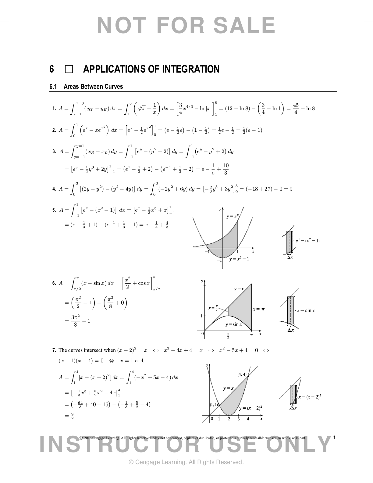
Buy this document to get the full access instantly
Instant Download Access after purchase
Add to cartInstant download
Reviews( 0 )
Document information
Connected school, study & course
About the document
Uploaded On
Jan 06, 2020
Number of pages
1
Written in

Additional information
This document has been written for:
Uploaded
Jan 06, 2020
Downloads
0
Views
39