Elements of Statistics. Chapter 1 to chapter 14 Exercise Solutions. All Answers 100% and Explained

Document Content and Description Below

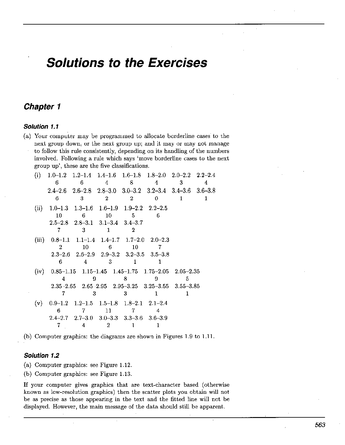
Exercise 4.1 m Assuming the cyclist's own estimate of '50 journeys a month' is accurate, what over the next month is the probability (a) that she never gets wet; (b) that she gets wet twice; (c)... that she gets wet at least four times? The cyclist's guess at a monthly average of 50 rides was just that-a guess. Suppose that a better estimate would have been 60 rides a month. In this case, using the given average 15 times per year, the estimated probability of a downpour during a single ride would be Exercise 4.2 The table following (Table 4.1) is half completed: it gives certain probabilities H DOD. for the binomial distribution B(50,1/40). From it, you could read off all your answers to Exercise 4.1. Complete the table by computing the corresponding probabilities for the binomial distribution B(60,1/48). Table 4.1 Probabilities, monthly downpours while cycling You will have noticed from Exercise 4.2 that the probabilities calculated for the cyclist but based on the higher estimate for cycle usage are not very different from those calculated for Exercise 4.1. To two decimal places, these values are identical. Exercise 4.3 (a) Write down the probability distribution of X , the number of errors per page, based on an estimate of 360 words per page and an average of 3.6 errors per page. (b) Calculate the probabilities px(0), p x (l), px(2), px (3) in this case, find the probability that there are more than three errors on a page, and comment on any differences in the results obtained between your model and the earlier binomial B(320,0.01125) 'guess'.Elements of Statistics In all these calculations, the binomial distribution has been used and the probability p has been 'rather small'. In Example 4.1, the results also suggested that for values of n not too different from one another, and with a corresponding estimate for the parameter p of 15 p=--- - 1.25 1 2 x n n ' probability calculations for the binomial distribution B(n, 1.25/n) did not differ significantly. (However, note that whatever the value of n, the mean of the distribution remains unaltered at p = np = 1.25.) Similarly, in Example 4.2, the actual value of n, at least in the two particular cases examined, was not too critical to the computed probabilities for the binomial distribution B(n, 3.6/n) (with constant mean 3.6). Now the question arises: can we satisfactorily model the number of monthly soakings for the cyclist, or the number of errors per page of proofs, using a random variable whose distribution depends only on a single parameter, the expected number? In general, can we approximate the two-parameter binomial distribution B(n, pln) by a probability distribution indexed by a single parameter p? The answer is that we can, provided p = p/n is small (which, in both these examples, it was) Use the recursive scheme defined by (4.3) to write down formulas for the probabilities ( a ) p x ( l ) , (b) P x P ) , (c) Px(3). Then (d) find a general expression for px (X). The definition of the Poisson distribution is as follows. The random variable X follows a Poisson distribution with parameter p if it has probability mass function It is easy to check that the function px(x) is indeed a probability functionthat is, that the terms sum to one. This vital property has not been lost in the derivation of the function from the binomial probability function. From the polynomial expansion Exercise 4.6 Resistors are very cheap electrical items, and they are easy to make. Assuming they work, they may be assumed to be indestructible. A small proportion (approximately 1 in 20) will not work when they leave the factory. This is a tolerable risk accepted by purchasers: these resistors are not quality tested before being packaged, for to do so would add considerably to their cost. (a) The resistors are boxed in packages of 50. State an 'exact' model for the number of defective resistors in a box, mentioning any assumptions you make and calculate the probabilities that there are 0, 1, 2, 3, 4 or more than 4 defectives in a box.- Chapter 4 Section 4.2 (b) Find an approximating distribution for the number of defectives in a box and calculate the same probabilities as you found in (a). (c) Comment on any differences between your answers in (a) and (b). This section ends with a final example where the Poisson model was useful. Exercise 4.7 This exercise is a computer simulation exercise designed to illustrate the results of this subsection. (a) use your computer to obtain a random sample of size five from the Poisson distribution with mean 8. List the elements of the sample, and find their mean. (b) Now obtain 100 samples of size five from the Poisson distribution with mean 8. In each case, calculate the sample mean, and store the 100 sample means in a data vector. (c) Plot a histogram of the data vector of part (b), and find its mean and variance. (d) Now repeat parts (b) and (c) but with samples of size fifty rather than five, and comment on any differences observed in the data vector of means. In Section 4.3 we shall look more closely at some general results for random variables. Exercise 4.8 (a) In Example 4.11 a random variable X with mean 40 was suggested as a model for the distribution of chest circumferences (measured in inches) amongst Scottish soldiers (based on historical data). What would be the mean circumference if the units of measurement were centimetres? This is one of the standard properties of a probability mass function. Earlier, we used the result E ( a X ) = a E ( X ) . (b) Suppose that in Example 4.12 the variation in water temperature was modelled by a probability distribution with mean 26 V. Find the mean temperature in degrees Fahrenheit.Chapter 4 Section 4.3 In order to work out the variance of the random variable a X + b, we shall start by writing Y = aX + b. The variance of Y is, by definition, V ( Y )= E [ ( Y- E(Y))'] and the expected value of Y is E ( Y ) = a E ( X )+ b from (4.11). So it follows that V ( Y )= E [ ( a X+ b- ( a E ( X )+ b))'] = E [ ( a X+b- a E ( X )- b)'] = E [ ( a X- ~ E ( x ) ) ~ ] = E [ a 2 ( x- E(x))'] (4.12) In (4.12) the expression ( X - E ( X ) ) ' is a random variable; a2 is a constant and can be taken outside the brackets. Thus V ( Y )= a 2 E [ ( x- E ( x ) ) ~ ] = a 2 v ( x ) . But Y is just the random variable aX + b, so we have obtained the result It follows from (4.13) (taking square roots of both sides) that S D ( a X + b) = da2V(X)= lalSD(X). (4.14) Notice that the constant b does not feature on the right-hand side of (4.13) or (4.14). The modulus sign in (4.14) is important since the constant a could be negative, but a standard deviation is always positive. Example 4.14 Sections of a chemical reactor Variation in the section temperature across the 1250 sections of a chemical reactor may be assumed to be adequately modelled by a normal distribution with mean 452 OC and standard deviation 22 deg C. From properties of the normal distribution we know that nearly all the recorded temperatures across the 1250 sections will lie within the range p - 30. to p + 30, or 386 "C to 518 OC. Converting from "C to OF leads to a new random variable with mean and standard deviation As it happens, this new random variable is also normally distributed: none of the preceding results imply this, but it is true nevertheless. You can probably appreciate that altering the scale of measurement will not alter the essential characteristics of the temperature variation: the probability density function reaches a peak at the mean temperature, tailing off symmetrically either side of the mean. See formula (3.9) in Chapter 3. Earlier, we used the result V ( a X )= a 2 v ( x ) . These are fictitious data based on a real investigation. See Cox, D.R. and Snell, E.J. (1981) Applied Statistics. Chapman and Hall, London, p. 68.Elements of Statistics Again, nearly all the temperatures across the sections of the reactor will lie within the range p - 3 ' ~ to p + 30: measured in "F the lower extreme is and the upper extreme is These could have been obtained in a different way by converting 386 "C and 518"C (the two likely temperature extremes) to "F. Exercise 4.9 In the early years of this century, statisticians were very concerned simply with the counting and measurement of random variables, and the recording of those measurements. Anything amenable to measurement and where there was evidence of variation was fair game. Some examples from issues of the journal Biometrika, from 1901 to 1902, include the number of sense organs of Aurelia Aurita; the number of ridges and furrows in the shells of different species of mollusc; the correlation between the number of stamens and the number of pistils in Ficaria ranunculoides during the flowering season; the dimensions of Hyalopterus trirhodus (aphids); the dimensions of the human skull; the dimensions of the egg of CUCUZUS Canorus (the cuckoo); the lengths of criminals' left middle fingers (and other dimensions); the number of sepals in Anemone nemorosa; the dimensions of the human hand; coat-colour in horses; the epidemiology of smallpox. A very large sample was used in assessing the variation in the lengths of criminals' left middle fingers: the variation may be very adequately modelled by a random variable X with mean 11.55cm and Macdonell, W.R. (1902) On standard deviation 0.55cm. criminal anthropometry and the identification of criminals. It is required for a comparison with Imperial measurements to make a trans- Biometrika, 1, 177-227. formation to inches. At l in = 2.54cm, what is the mean and standard deviation in the new scale? These results for moments of a linear function of a random variable X may be summarized as follows. If X is a random variable with mean px and standard deviation 'JX, and if the random variable Y is defined by Y = a X + b , where a and b are constants, then Y has moments This section ends with a result which provides a very useful alternative formula for the variance of a random variable X. 162Chapter 4 Section 4.3 First, we shall need the incidental result that if hl(X) and h2(X) are two functions of a random variable X , then the expected value of their sum is equal to the sum of their expected values: This is easy to check. In the case that X is discrete, for instance, having probability mass function p(%),then Similar manipulations will confirm (4.15) when X is a continuous random variable. The formula we have been using so far for the variance of a random variable X with expected value p is Expanding the square on the right-hand side gives The expression X 2- 2pX + p2 can be written in the form hl(X) + h2(X) in more than one way, but the most useful way is to set hl(X) =x2and h2(X)= (-2pX + p2). Then it follows that Furthermore, we can apply our formula for the mean of a linear function of X , E ( a X + b) = aE(X) + b, to the last term above. Setting a = -2p and b = p2 we finally obtain the result This formulation is sometimes easier to implement than the formula for the variance that we have used up to now.Elements of Statistics Example 4.15 A perfect die In Chapter 3 , page 110 you saw that the random variable X with probability mass function (used as a probability model for the outcome of throws of a perfectly engineered die) has mean and variance Using the alternative formula (4.16) for the variance we first need the value of E(X2): this is Then 2 V(X) = E ( X ) - p2 = F- ( 3 . ~ ) ~ = - = E = 2.92 as before. Exercise 4.10 In Chapter 3 Exercise 3.7, you showed that the variance in the outcome of 1 rolls of a Double-Five was 1616 = 2.7. (The.mean outcome is 4.) Confirm this result for the variance using the formula (4.16). It was earlier remarked that, in general, exact distributional results for random samples are rather difficult to obtain. There are some exceptions to this rule, four of which we shall now briefly explore. Exercise 4.1 1 You saw in Chapter 3, Example 3.5, that if X is binomial B(4,0.4) then the individual probabilities for X are as follows. X 0 1 2 3 4 p(x) 0.1296 0.3456 0.3456 0.1536 0.0256 Use the formulas at (4.17) to write down the mean and variance of X and confirm your result for the variance of X using the result V(X) = E(x2) - (E(x))~ obtained at (4.16). B Sums of Poisson random variables If Xi, i = 1,2,...,n, are independent Poisson variates with respective means pi, then their sum Y = X1 + X2+ . . .+ X, is also a Poisson variate, with mean p1 + p2+ . e + p,: that is, Y Poisson(pl + p2+ . ..f pn). (4.18) This result is stated without proof. Notice that, given the distributions of the independent components Xi, you could have written down the mean and the variance of Y immediately using results (4.7) and (4.9). What is not obvious is that the distribution of the sum Y = XI + X2+ . .+ Xn is also Poisson.Elements of Statistics (Incidentally, notice that the result is quite general: there is no requirement here, as there is in the case of a random sample, that the Xis should be identically distributed, only that they should be independent.) Exercise 4.12 m What would the geometric model give for the probability of a time lag between B earthquakes exceeding four years? How many cases are there of such a lull being recorded? Exercise 4.13 Assume that earthquakes occur world-wide at random but at an estimated average rate of once every 437 days. Assuming a continuous-time model for the phenomenon, find (a) the probability that no earthquake is experienced world-wide during the first three years of the third millenium (that is, during the years 2000-2002 inclusive. The year 2000 will be a leap year); (b) the median time between successive earthquakes (that is, the solution X of the equation F(x) = i); (c) the proportion of waiting times longer than expected (that is, the proportion of waiting times that exceed 437 days). You saw from your answer to Exercise 4.13(b) that the median of the exponential distribution is very much less than the mean. Figure 4.4 is reproduced here as Figure 4.5 with A set equal to 11437: it shows the median and mean waiting time between earthquakes, and the probability you calculated in Exercise 4.13(c). Exercise 4.14 Assuming that in a typical decade the expected number of earthquakes world- 1 wide is 8.35, find the probability that there will be (a) exactly two earthquakes; (b) at least four earthquakes. Exercise 4.15 Express the median waiting time between consecutive events in a Poisson H process as a fraction of the mean waiting time. Exercise 4.16 (a) Assuming the mean time between earthquakes to be 437 days as suggested by the data in Table 4.6, use your computer to simulate the times of earthquakes world-wide over a twenty-year period. (Ignore leap years: assume 365 days a year.) List the times of occurrence in a table, and on a diagram represent the incidence of earthquakes against time. (b) How many earthquakes were there in your simulation? How many should you have expected? What is the median number of earthquakes to occur world-wide in a twenty-year period? Exercise 4.16 (a) Assuming the mean time between earthquakes to be 437 days as suggested by the data in Table 4.6, use your computer to simulate the times of earthquakes world-wide over a twenty-year period. (Ignore leap years: assume 365 days a year.) List the times of occurrence in a table, and on a diagram represent the incidence of earthquakes against time. (b) How many earthquakes were there in your simulation? How many should you have expected? What is the median number of earthquakes to occur world-wide in a twenty-year period? Here is a final exercise covering the main points of the section. Exercise 4.17 Here, our aim is to develop an adequate model for the following data set. The data in Table 4.10 give the time intervals (in seconds) between successive pulses along a nerve fibre. They are extracted from a large data set in which there were 800 pulses recorded, so there were 799 waiting times between pulses. Cox, D.R. and Lewis, P.A.W. The data in Table 4.10 are the first 200 waiting times. (1966) The Statistical Analysis of Series o f Events. Chapman and Table 4.10 Waiting times between pulses (seconds) 0.21 0.03 0.05 0.11 0.59 0.06 0.18 0.55 0.37 0.14 0.19 0.02 0.14 0.09 0.05 0.15 0.23 0.15 0.24 0.16 0.06 0.11 0.15 0.09 0.03 0.21 0.02 0.24 0.29 0.16 0.07 0.07 0.04 0.02 0.15 0.12 0.15 0.33 0.06 0.51 0.11 0.28 0.36 0.14 0.55 0.04 0.01 0.94 0.73 0.05 0.07 0.11 0.38 0.21 0.38 0.38 0.01 0.06 0.13 0.06 0.01 0.16 0.05 0.16 0.06 0.06 0.06 0.06 0.11 0.44 0.05 0.09 0.27 0.50 0.25 0.25 0.08 0.01 0.70 0.04 0.08 0.38 0.08 0.32 0.39 0.58 0.56 0.74 0.15 0.07 0.25 0.01 0.17 0.64 0.61 0.15 0.26 0.03 0.05 0.07 0.10 0.09 0.02 0.30 0.07 0.12 0.01 0.16 0.49 0.07 0.11 0.35 1.21 0.17 0.01 0.35 0.45 0.93 0.04 0.96 0.14 1.38 0.15 0.01 0.05 0.23 0.05 0.05 0.29 0.01 0.74 0.30 0.09 0.02 0.19 0.01 0.51 0.12 0.12 0.43 0.32 0.09 0.20 0.03 0.13 0.15 0.05 0.08 0.04 0.09 0.10 0.10 0.26 0.68 0.15 0.01 0.27 0.05 0.03 0.40 0.04 0.21 0.24 0.08 0.23 0.10 0.19 0.20 0.26 0.06 0.40 0.15 1.10 0.16 0.78 0.04 0.27 0.35 0.71 0.15 Plot a histogram of these data and comment on the shape of your diagram. Compare (i) the sample mean with the sample median; (ii) the sample mean with the sample standard deviation. Find the lower and upper quartiles for the exponential distribution (expressed in terms of the mean) and compare these with the sample upper and lower quartiles for these data. Count the number of pulses to have occurred during the first quarterminute of observation. (Assume the first pulse to have occurred at time zero when the clock was started, so that the first pulse recorded occurred Hall, ~ o i d o n , p. 252. - ~ a t a provided by Dr. P. Fatt and Professor B. Katz, F.R.S., University College London.Elements of Statistics at time 0.21, the second at time 0.21+ 0.03 = 0.24, and so on.) How many occurred during the second quarter-minute? Your answers to parts (a) to (c) may have enabled you to formulate a model for the incidence of pulses along a nerve fibre. (e) Assuming your model to be correct, from what probability distribution are the counts you wrote down in part (d) observations? Here is a final example, one where the model assumptions broke down. Example 4.19 Admissions to an intensive care unit Data were collected on the arrival times of patients at an intensive care unitthe aim was to identify any systematic variations in arrival rate, in particular, any that might be useful in planning future management of the unit. Cox, D.R. and Snell, E.J. (1981) Table 4.11 gives some of these data. It might initially be supposed that ad- Chapman and Hall, London, p. 53. Data collected missions occur in the 'random haphazard' way suggested in the earthquake by Dr. A, Barr, Oxford Regiollal example. In fact, there are noticeable variations in the data that cannot be ~ ~ ~ ~ i t ~ l ascribed simply to chance variation on the exponential distribution. These are due to variations in the underlying rate of admission both with the time of day and with the day of the week. (The original data give the day and time of admission. Differences have been taken to give the inter-admission waiting times, to the nearest half-hour. The time of observation was from 4 February 1963 to 9 May 1963.) Exercise 4.18 The aim here is to compare a random sample of observations with the theoretical frequencies for the Poisson distribution. (a) Generate 20 observations from the Poisson distribution Poisson(3.2) and then tally the data. Repeat the exercise for 50 observations and then 100 observations. (b) Now generate 1000observations from the Poisson distribution Poisson(3.2), obtain sample relative frequencies, and compare these with the probability mass function for a Poisson random variable with mean 3.2. Exercise 4.19 Suppose that in an assembly of 100 persons the number of males X is a random variable B(100,0.5). Simulate the number of males in the assembly and hence deduce the number of females. Say there are X males. Using an exact binomial model (rather than the Poisson approximation) with p = 0.06 sinlulate the number of colourdeficient males (yl) and similarly the number of colour-deficient females (y2) present. Their sum W = yl + yz is an observation on a random variable W, the total number of colour-deficient people in an assembly of 100. Find W in this case. The distribution of W is unknown, a rather complex conjunction of binomial variates.Chapter 4 Section 4.5 (d) On intuitive grounds alone (that is, without stopping to think too hard!) can you say anything about the expected value of W? (e) Obtain 1000 independent observations wl, w2, . ..,wlooo on the random variable W and store them in a data vector. Calculate the sample mean and variance of this random sample. Exercise 4.20 The times of occurrence of random unforecastable events such as car accidents or floods may be modelled by assuming that the waiting times between consecutive occurrences come from an exponential distribution with some given mean: that is, that such events occur as a Poisson process. Adding successive waiting times gives the times at which such accidents might typically occur. (a) Suppose that motor accident claims of a particular kind arrive at an underwriter's office in a way which is not forecastable, but at an average rate of twelve claims a week. (Assume for the sake of this exercise that the office is open for business 24 hours a day, seven days a week.) Calculate the mean time (in hours) between the arrival of successive claims. Simulate the times of arrival of the next 20 claims to arrive after midnight one Sunday night. (b) Simulate ten weeks of claims. How many claims arrived in the first week? The second week? ... The tenth week? These ten counts are observations on what random variable? [Show More]

Last updated: 1 year ago

Preview 1 out of 105 pages