ISYE6501 HOMEWORK 10, Questions with accurate answers, Graded A+

Document Content and Description Below

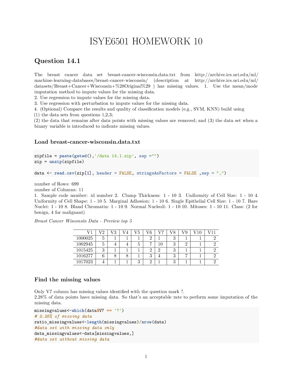
ISYE6501 HOMEWORK 10 Question 14.1 The breast cancer data set breast-cancer-wisconsin.data.txt from http://archive.ics.uci.edu/ml/ machine-learning-databases/breast-cancer-wisconsin/ (description a... t http://archive.ics.uci.edu/ml/ datasets/Breast+Cancer+Wisconsin+%28Original%29 ) has missing values. 1. Use the mean/mode imputation method to impute values for the missing data. 2. Use regression to impute values for the missing data. 3. Use regression with perturbation to impute values for the missing data. 4. (Optional) Compare the results and quality of classification models (e.g., SVM, KNN) build using (1) the data sets from questions 1,2,3; (2) the data that remains after data points with missing values are removed; and (3) the data set when a binary variable is introduced to indicate missing values. Load breast-cancer-wisconsin.data.txt zipfile = paste(getwd(),'/data 14.1.zip', sep ="") zip = unzip(zipfile) data <- read.csv(zip[1], header = FALSE, stringsAsFactors = FALSE ,sep = ",") number of Rows: 699 number of Columns: 11 1. Sample code number: id number 2. Clump Thickness: 1 - 10 3. Uniformity of Cell Size: 1 - 10 4. Uniformity of Cell Shape: 1 - 10 5. Marginal Adhesion: 1 - 10 6. Single Epithelial Cell Size: 1 - 10 7. Bare Nuclei: 1 - 10 8. Bland Chromatin: 1 - 10 9. Normal Nucleoli: 1 - 10 10. Mitoses: 1 - 10 11. Class: (2 for benign, 4 for malignant) Breast Cancer Wisconsin Data - Preview top 5 V1 V2 V3 V4 V5 V6 V7 V8 V9 V10 V11 1000025 5 1 1 1 2 1 3 1 1 2 1002945 5 4 4 5 7 10 3 2 1 2 1015425 3 1 1 1 2 2 3 1 1 2 1016277 6 8 8 1 3 4 3 7 1 2 1017023 4 1 1 3 2 1 3 1 1 2 Find the missing values Only V7 column has missing values identified with the question mark ?. 2.28% of data points have missing data. So that’s an acceptable rate to perform some imputation of the missing data. missingvalues<-which(data$V7 == '?') # 2.28% of missing data ratio_missingvalues<-length(missingvalues)/nrow(data) #data set with missing data only data_missingvalues<-data[missingvalues,] #data set without missing data 1data_no_missingvalues<-data[-missingvalues,] data_no_missingvalues$V7 = as.integer(data_no_missingvalues$V7) Does the missing values have any bias? Since the goal is to predict V11, One quick way to verify whether the missing values are carrying any bias, is to compare the distribution of V11’s values in the population with missing values and the distribution in the population without missing values. V11 = 2 represent 87.5% of the missing value data set versus 65% in the data set without missing value. So we might conclude that the missing value population might have some bias. #0.6552217 sum(data$V11 == 2)/nrow(data) ## [1] 0.6552217 #0.875 sum(data_missingvalues$V11 == 2)/nrow(data_missingvalues) ## [1] 0.875 #0.6500732 sum(data_no_missingvalues$V11 == 2)/nrow(data_no_missingvalues) ## [1] 0.6500732 1. Use the mean/mode imputation method to impute values for the missing data. Mode imputation is prefered for categorical variables. In our case, V7 is apparently an ordinal variable so we might consider to treat it as a categorical or continuous variable. I will use both methods mean and mode imputations, and I will create one column for the mean imputation and one column for the mode imputation to imputethe missing values of V7. One quick comment: taking the mean might give us a float; I arbitrary rounding the value to the nearest integer. # Compute the mean on the non missing values of V7 mean_V7<-round(mean(as.integer(data_no_missingvalues$V7))) #mean: 3.544656 => mean_V7: 4 new_data<-data new_data$mean<-new_data$V7 new_data$mean[new_data$mean== "?"] <- round(mean_V7) new_data$mean<-as.numeric(new_data$mean) # Create the function. getmode <- function(v) { uniqv <- unique(v) uniqv[which.max(tabulate(match(v, uniqv)))] } # Calculate the mode using the user function. #mode_V7 = 1 mode_V7 <- getmode(as.integer(data_no_missingvalues$V7)) 2# new_data$mode<-new_data$V7 new_data$mode[new_data$mode== "?"] <- mode_V7 new_data$mode<-as.integer(new_data$mode) V7 mean value is 4 and the V7 mode value is 1. Both have distinctive values and that might gives different prediction result if V7 is used in the model to predict V11. 2. Use regression to impute values for the missing data. I will use Elastic Net and run a cross validation to identify the best alpha, lambda for selecting my model. I used that method in the homework 8. Training and Testing Sets. For training and validation, I selected 80% of the data excluding the data points with missing V7 values. set.seed(11) train_size = as.integer(nrow(data_no_missingvalues)*0.8) train_ind <- sample(seq_len(nrow(data_no_missingvalues)), size = train_size) df_train <- data_no_missingvalues[train_ind, ] df_test <- data_no_missingvalues[-train_ind, ] Elastic Net - Cross validation I am training the Elastic Net regression on various values of alpha to estimate V7. V7’s prediction is also rounded to the nearest integer. I will select the best model(alpha and lambda) based on the best R-squared and/or Mean Square Error MSE. Lets make sure to exclude V11 from the model to minimize overfitting when we train the model to predict V11. I also excluded V1 since its an ID and not a factor. x <- df_train x$V1<-NULL x$V7<-NULL x$V11<-NULL x <- as.matrix(x) y <- df_train$V7 models <- data.frame(alpha=numeric(), lambda=numeric(), mse=numeric(), R2=numeric()) for (i in 0:20) { alpha = i/20 set.seed(11) cv.model.elastic = cv.glmnet(x,y, family="gaussian", type.measure="mse", nfolds=4, standardize=TRUE, alpha=alpha) 3lambda = cv.model.elastic$lambda.1se model.elastic = glmnet(x,y, family="gaussian", standardize=TRUE, alpha=alpha, lambda=lambda) model.elastic.yhat = round(predict(model.elastic, s = lambda, newx = x, type = "response")) mse <- mean((y - model.elastic.yhat)^2) SSres <- sum((model.elastic.yhat-y)^2) SStot <- sum((y - mean(y))^2) model.elastic.R2 <- 1 - SSres/SStot model <- data.frame(alpha = alpha, lambda = lambda, mse = mse, R2 = model.elastic.R2) models <- rbind(models, model) } plot(models$alpha,models$mse,type = "b") 0.0 0.2 0.4 0.6 0.8 1.0 5.50 5.55 5.60 5.65 models$alpha models$mse best_R2 = max(models$R2) #0.60 best_mse<-models[models$R2==best_R2,]$mse #5.42 best_alpha<-models[models$R2==best_R2,]$alpha #0.45 best_lambda<-models[models$R2==best_R2,]$lambda #0.907 The model with the best(highest) R-square = 0.5835256 and MSE = 5.4981685 has alpha = 0.5 and lambda = 0.9042212. Elastic Net - Model Test Let’s train the final Elastic Net regression model using the best alpha = 0.5 and lambda = 0.9042212. model.elastic = glmnet(x,y, family="gaussian", [Show More]

Last updated: 1 year ago

Preview 1 out of 10 pages